
中文
训练电池 AI 实例:用 PyBaMM 仿真数据预测 SOH 与 RUL
前述架构已经建立了利用 PyBaMM 生成基于物理的阻抗 (EIS) 张量的完整数据流。现在我们将进入电池信息学中最核心且最受学术界审视的阶段:训练序列到序列的深度学习模型(如 LSTMs, Transformers)来预测健康状态 (SOH) 与剩余使用寿命 (RUL)。我们抛弃了简单的特征工程,转而研究将高维电化学状态直接映射到电池生命周期轨迹的方法。
由严谨的 DFN/SPMe 模型生成的基于物理的合成样本,对于预训练物理信息神经网络 (PINN) 和验证状态估计器协方差矩阵具有不可估量的价值,但在最终应用时严格需要与实际电芯退化路径进行标定对齐。
一、退化动力学的随机过程建模
电池老化是一个非马尔可夫 (non-Markovian) 过程;在循环 $k$ 时的内部状态取决于整个生命周期的应力历史。在最优估计理论的框架下,SOH 和 RUL 被视为离散时间非线性动力系统中的不可见隐状态。用于 SOH 追踪的经典表示方法通常采用扩展卡尔曼滤波 (EKF) 公式:
状态转移模型(包含 SEI 增厚与活性物质损失):
$$ x_{k+1} = f(x_k, u_k) + w_k, quad w_k sim mathcal{N}(0, Q) $$
观测模型(EIS 谱图与端电压极限):
$$ y_k = h(x_k, u_k) + v_k, quad v_k sim mathcal{N}(0, R) $$
这里,$x_k$ 封装了直接对应于 SOH 的内部容量参数(如 LLI、LAM)。我们的深度学习任务,就是用参数为 $theta$ 的可微神经网络替换掉传统的启发式观测函数 $h(cdot)$,从而最大化退化轨迹的联合对数似然。
二、用于预测预测的深度序列架构
为了捕获容量衰减的长期时序依赖性以及非线性“跳水点” (knee point) 的确切发生时机,我们实现了 Transformer 编码器架构。与基础的前馈网络不同,注意力机制天生具备处理 Nyquist 张量可变长度循环历史的能力。
import torch
import torch.nn as nn

class ImpedanceTransformer(nn.Module):
    def __init__(self, input_dim=120, d_model=256, nhead=8, num_layers=4):
        super().__init__()
        # 将原始 EIS 张量 (实部、虚部数组) 投影到隐空间
        self.input_projection = nn.Linear(input_dim, d_model)

        # 针对循环次数的位置编码
        self.pos_encoder = PositionalEncoding(d_model)

        # 处理时序退化特征的 Transformer 编码器
        encoder_layers = nn.TransformerEncoderLayer(d_model=d_model, nhead=nhead, batch_first=True)
        self.transformer = nn.TransformerEncoder(encoder_layers, num_layers=num_layers)

        # 多任务输出头:SOH 连续回归与 RUL 期望
        self.soh_head = nn.Linear(d_model, 1)
        self.rul_head = nn.Sequential(
            nn.Linear(d_model, 64),
            nn.GELU(),
            nn.Linear(64, 1),
            nn.Softplus() # RUL 必须是严格的正数
        )

    def forward(self, eis_sequence):
        # eis_sequence 维度: [batch_size, sequence_length, input_dim]
        x = self.input_projection(eis_sequence)
        x = self.pos_encoder(x)
        features = self.transformer(x)

        # 提取最新循环的特征用于最终预测
        latest_features = features[:, -1, :]
        soh_pred = self.soh_head(latest_features)
        rul_pred = self.rul_head(latest_features)

        return soh_pred, rul_pred
输入张量由标准化对数频率空间下的实部 $Z_{re}(omega)$ 和虚部 $Z_{im}(omega)$ 级联而成,并融合了操作应力因子(如温度 $T$、放电深度 $Delta DOD$、充放电倍率 $C$-rate)。
三、损失曲面的正则化
在电池寿命早期直接预测 RUL 本质上是一个不适定 (ill-posed) 问题。我们采用包含物理信息正则化的多任务范式来构建损失函数 $mathcal{L}(theta)$:
$$ mathcal{L}(theta) = lambda_1 | text{SOH}_{pred} - text{SOH}_{true} |_2^2 + lambda_2 text{Huber}(text{RUL}_{pred}, text{RUL}_{true}) + lambda_3 Phi(x) $$
其中,惩罚项 $Phi(x)$ 用于强制施加物理单调性约束(例如,排除静置恢复现象后,SOH 必须是严格单调递减的)。
四、对抗协变量偏移与数据泄漏
在合成数据机器学习中,最致命的错误就是执行逐行的独立随机拆分。从单个 PyBaMM Simulation.solve() 轨迹中派生的时间序列数据具有完全确定性的协方差。如果同一电芯的第 $N$ 次循环和第 $N+1$ 次循环分别落入训练集和测试集,Transformer 会轻易通过线性插值“作弊”完成预测任务,这将导致模型在部署到实际硬件时发生灾难性的泛化失败。
我们必须通过使用 cell_design_id 或 protocol_id 在参数空间的正交维度上对拆分进行分层,来强制执行严格的分布外 (OOD) 交叉验证:
from sklearn.model_selection import GroupKFold

# 完全依据确定性的物理配置组进行拆分
gkf = GroupKFold(n_splits=5)
for train_idx, test_idx in gkf.split(X, y, groups=metadata["cell_design_id"]):
    train_tensor = X[train_idx]
    # 执行 PyTorch 训练循环
五、向 BMS 微控制器部署的工程挑战
真实的 BMS 依赖于算力不足 100 MHz 且具备 ASIL 安全等级的车规级 MCU。在 PyTorch 中训练出的庞大且包含多头注意力权重的模型必须经过极端的压缩。我们利用训练后量化 (PTQ) 技术将其转换为 Int8 精度,并结合结构化剪枝去除了 95% 的模型体积。残余的高效网络通过 ONNX 导出,与底层的 C++ 推理引擎集成,并部署在硬件 EKF 矩阵数学运算模块旁运行。
References
英文
Training a Battery AI Model with PyBaMM: Predicting SOH and RUL
在独立页面打开The previous architecture established the pipeline for generating physics-based Impedance (EIS) tensors via PyBaMM. We now pivot to the most heavily scrutinized step in battery informatics: training sequence-to-sequence deep learning models (LSTMs, Transformers) to predict State of Health (SOH) and Remaining Useful Life (RUL). We discard simplistic feature-engineering in favor of mapping high-dimensional electrochemical states to prognostic life trajectories.
Physics-based synthetic samples generated by rigorous DFN/SPMe formulations are invaluable for pretraining Physics-Informed Neural Networks (PINNs) and validating estimator covariance matrices, but they strictly necessitate eventual alignment with empirical cell degradation paths.
1. The Stochastic Degradation Dynamics
Battery aging is non-Markovian; the internal state at cycle $k$ depends on the entire stress history. In the context of optimal estimation theory, the SOH and RUL are treated as unobserved latent states within a discrete-time nonlinear dynamical system. A canonical representation for SOH tracking utilizes the Extended Kalman Filter (EKF) formulation:
State transition model (incorporating SEI thickening and active material loss):
$$ x_{k+1} = f(x_k, u_k) + w_k, quad w_k sim mathcal{N}(0, Q) $$
Observation model (EIS spectra and terminal voltage limits):
$$ y_k = h(x_k, u_k) + v_k, quad v_k sim mathcal{N}(0, R) $$
Where $x_k$ encapsulates the internal capacity parameters (LLI, LAM) corresponding to SOH. Our deep learning task replaces the heuristic observation function $h(cdot)$ with a differentiable neural network parameterized by $theta$, optimizing the joint log-likelihood of the degradation trajectory.
2. Deep Sequence Architectures for Prognostics
To capture the long-term temporal dependencies of capacity fade and the specific onset of the nonlinear "knee" point, we implement a Transformer encoder architecture. Unlike basic feed-forward networks, attention mechanisms natively process the variable-length cycle histories of Nyquist tensors.
import torch
import torch.nn as nn

class ImpedanceTransformer(nn.Module):
    def __init__(self, input_dim=120, d_model=256, nhead=8, num_layers=4):
        super().__init__()
        # Project raw EIS tensors (Re, Im arrays) into latent space
        self.input_projection = nn.Linear(input_dim, d_model)

        # Positional encoding for cycle number
        self.pos_encoder = PositionalEncoding(d_model)

        # Transformer Encoder processing temporal degradation
        encoder_layers = nn.TransformerEncoderLayer(d_model=d_model, nhead=nhead, batch_first=True)
        self.transformer = nn.TransformerEncoder(encoder_layers, num_layers=num_layers)

        # Multi-task head: SOH regression and RUL expectation
        self.soh_head = nn.Linear(d_model, 1)
        self.rul_head = nn.Sequential(
            nn.Linear(d_model, 64),
            nn.GELU(),
            nn.Linear(64, 1),
            nn.Softplus() # RUL is strictly positive
        )

    def forward(self, eis_sequence):
        # eis_sequence shape: [batch_size, sequence_length, input_dim]
        x = self.input_projection(eis_sequence)
        x = self.pos_encoder(x)
        features = self.transformer(x)

        # Extract features from the latest cycle for prediction
        latest_features = features[:, -1, :]
        soh_pred = self.soh_head(latest_features)
        rul_pred = self.rul_head(latest_features)

        return soh_pred, rul_pred
The input tensor comprises concatenated real and imaginary components $Z_{re}(omega)$ and $Z_{im}(omega)$ across a standardized frequency log-space, combined with operational stress factors ($T$, $Delta DOD$, $C$-rate).
3. Regularizing the Loss Surface
Predicting RUL directly is fundamentally ill-posed early in life. We structure the loss function $mathcal{L}(theta)$ using a multi-task paradigm with physics-informed regularization:
$$ mathcal{L}(theta) = lambda_1 | text{SOH}_{pred} - text{SOH}_{true} |_2^2 + lambda_2 text{Huber}(text{RUL}_{pred}, text{RUL}_{true}) + lambda_3 Phi(x) $$
Where $Phi(x)$ enforces physical monotonicity constraints (e.g., SOH strictly monotonically decreasing barring relaxation phenomena).
4. Combating Covariate Shift and Leakage
The cardinal sin in synthetic data ML is row-wise independent splitting. Time-series data derived from a singular PyBaMM Simulation.solve() trajectory exhibits deterministic covariance. If cycle $N$ and cycle $N+1$ from the same cell fall into train and test sets respectively, the Transformer trivializes the prediction task via linear interpolation, yielding a catastrophic generalization failure when deployed on hardware.
We enforce strict out-of-distribution (OOD) cross-validation by stratifying the splits across orthogonal dimensions of the parameter space using cell_design_id or protocol_id:
from sklearn.model_selection import GroupKFold

# Splitting purely by deterministic physical configurations
gkf = GroupKFold(n_splits=5)
for train_idx, test_idx in gkf.split(X, y, groups=metadata["cell_design_id"]):
    train_tensor = X[train_idx]
    # Execute PyTorch training loop
5. Deploying to BMS Microcontrollers
A real-world BMS relies on ASIL-rated MCUs computing at sub-100 MHz. The massive multi-headed attention weights developed in PyTorch must be aggressively compressed. We utilize post-training quantization (PTQ) to Int8 and structural pruning to strip 95% of the model footprint. The residual network is exported via ONNX, integrated with an embedded C++ inference engine, and deployed adjacent to the hardware EKF matrix math.
References
前述架构已经建立了利用 PyBaMM 生成基于物理的阻抗 (EIS) 张量的完整数据流。现在我们将进入电池信息学中最核心且最受学术界审视的阶段:训练序列到序列的深度学习模型(如 LSTMs, Transformers)来预测健康状态 (SOH) 与剩余使用寿命 (RUL)。我们抛弃了简单的特征工程,转而研究将高维电化学状态直接映射到电池生命周期轨迹的方法。
由严谨的 DFN/SPMe 模型生成的基于物理的合成样本,对于预训练物理信息神经网络 (PINN) 和验证状态估计器协方差矩阵具有不可估量的价值,但在最终应用时严格需要与实际电芯退化路径进行标定对齐。
一、退化动力学的随机过程建模
电池老化是一个非马尔可夫 (non-Markovian) 过程;在循环 $k$ 时的内部状态取决于整个生命周期的应力历史。在最优估计理论的框架下,SOH 和 RUL 被视为离散时间非线性动力系统中的不可见隐状态。用于 SOH 追踪的经典表示方法通常采用扩展卡尔曼滤波 (EKF) 公式:
状态转移模型(包含 SEI 增厚与活性物质损失):
$$ x_{k+1} = f(x_k, u_k) + w_k, quad w_k sim mathcal{N}(0, Q) $$
观测模型(EIS 谱图与端电压极限):
$$ y_k = h(x_k, u_k) + v_k, quad v_k sim mathcal{N}(0, R) $$
这里,$x_k$ 封装了直接对应于 SOH 的内部容量参数(如 LLI、LAM)。我们的深度学习任务,就是用参数为 $theta$ 的可微神经网络替换掉传统的启发式观测函数 $h(cdot)$,从而最大化退化轨迹的联合对数似然。
二、用于预测预测的深度序列架构
为了捕获容量衰减的长期时序依赖性以及非线性“跳水点” (knee point) 的确切发生时机,我们实现了 Transformer 编码器架构。与基础的前馈网络不同,注意力机制天生具备处理 Nyquist 张量可变长度循环历史的能力。
import torch
import torch.nn as nn

class ImpedanceTransformer(nn.Module):
    def __init__(self, input_dim=120, d_model=256, nhead=8, num_layers=4):
        super().__init__()
        # 将原始 EIS 张量 (实部、虚部数组) 投影到隐空间
        self.input_projection = nn.Linear(input_dim, d_model)

        # 针对循环次数的位置编码
        self.pos_encoder = PositionalEncoding(d_model)

        # 处理时序退化特征的 Transformer 编码器
        encoder_layers = nn.TransformerEncoderLayer(d_model=d_model, nhead=nhead, batch_first=True)
        self.transformer = nn.TransformerEncoder(encoder_layers, num_layers=num_layers)

        # 多任务输出头:SOH 连续回归与 RUL 期望
        self.soh_head = nn.Linear(d_model, 1)
        self.rul_head = nn.Sequential(
            nn.Linear(d_model, 64),
            nn.GELU(),
            nn.Linear(64, 1),
            nn.Softplus() # RUL 必须是严格的正数
        )

    def forward(self, eis_sequence):
        # eis_sequence 维度: [batch_size, sequence_length, input_dim]
        x = self.input_projection(eis_sequence)
        x = self.pos_encoder(x)
        features = self.transformer(x)

        # 提取最新循环的特征用于最终预测
        latest_features = features[:, -1, :]
        soh_pred = self.soh_head(latest_features)
        rul_pred = self.rul_head(latest_features)

        return soh_pred, rul_pred
输入张量由标准化对数频率空间下的实部 $Z_{re}(omega)$ 和虚部 $Z_{im}(omega)$ 级联而成,并融合了操作应力因子(如温度 $T$、放电深度 $Delta DOD$、充放电倍率 $C$-rate)。
三、损失曲面的正则化
在电池寿命早期直接预测 RUL 本质上是一个不适定 (ill-posed) 问题。我们采用包含物理信息正则化的多任务范式来构建损失函数 $mathcal{L}(theta)$:
$$ mathcal{L}(theta) = lambda_1 | text{SOH}_{pred} – text{SOH}_{true} |_2^2 + lambda_2 text{Huber}(text{RUL}_{pred}, text{RUL}_{true}) + lambda_3 Phi(x) $$
其中,惩罚项 $Phi(x)$ 用于强制施加物理单调性约束(例如,排除静置恢复现象后,SOH 必须是严格单调递减的)。
四、对抗协变量偏移与数据泄漏
在合成数据机器学习中,最致命的错误就是执行逐行的独立随机拆分。从单个 PyBaMM Simulation.solve() 轨迹中派生的时间序列数据具有完全确定性的协方差。如果同一电芯的第 $N$ 次循环和第 $N+1$ 次循环分别落入训练集和测试集,Transformer 会轻易通过线性插值“作弊”完成预测任务,这将导致模型在部署到实际硬件时发生灾难性的泛化失败。
我们必须通过使用 cell_design_id 或 protocol_id 在参数空间的正交维度上对拆分进行分层,来强制执行严格的分布外 (OOD) 交叉验证:
from sklearn.model_selection import GroupKFold

# 完全依据确定性的物理配置组进行拆分
gkf = GroupKFold(n_splits=5)
for train_idx, test_idx in gkf.split(X, y, groups=metadata["cell_design_id"]):
    train_tensor = X[train_idx]
    # 执行 PyTorch 训练循环
五、向 BMS 微控制器部署的工程挑战
真实的 BMS 依赖于算力不足 100 MHz 且具备 ASIL 安全等级的车规级 MCU。在 PyTorch 中训练出的庞大且包含多头注意力权重的模型必须经过极端的压缩。我们利用训练后量化 (PTQ) 技术将其转换为 Int8 精度,并结合结构化剪枝去除了 95% 的模型体积。残余的高效网络通过 ONNX 导出,与底层的 C++ 推理引擎集成,并部署在硬件 EKF 矩阵数学运算模块旁运行。
References
搜索问题
常见问题
这篇文章适合谁读?
这篇文章适合想用 博士生 难度理解“训练电池 AI 实例:用 PyBaMM 仿真数据预测 SOH 与 RUL”的读者,预计阅读时间约 14 分钟,重点覆盖 PyBaMM, scikit-learn, SOH, RUL。
读完后下一步应该看什么?
可以从文末相关阅读、项目页和知识图谱继续进入相邻主题。
这篇文章有没有可运行代码或配套资源?
有。页面里的运行说明、资源卡片和下载入口会指向复现实验所需的命令、数据、代码或说明文件。
这篇文章和整个网站的学习路线有什么关系?
它会通过文章上下文、学习路线、资源库和项目时间线连接到同一主题下的其他内容。
文章上下文
电池建模与 AI
围绕 PyBaMM、EIS、老化仿真和 AI 标签数据,建立可复查的物理建模到机器学习数据管线。
配套资源
电池建模与 AI / DATASET
SOH/RUL 训练指标 CSV
保存 group split、MAE、RMSE、R2、label source 和 backend used,用于复查训练结果。
电池建模与 AI / DATASET
SOH/RUL held-out 预测 CSV
保存测试样本的真实值、预测值和绝对误差。
电池建模与 AI / DATASET
SOH/RUL 特征重要性 CSV
记录每个目标模型的随机森林特征重要性。
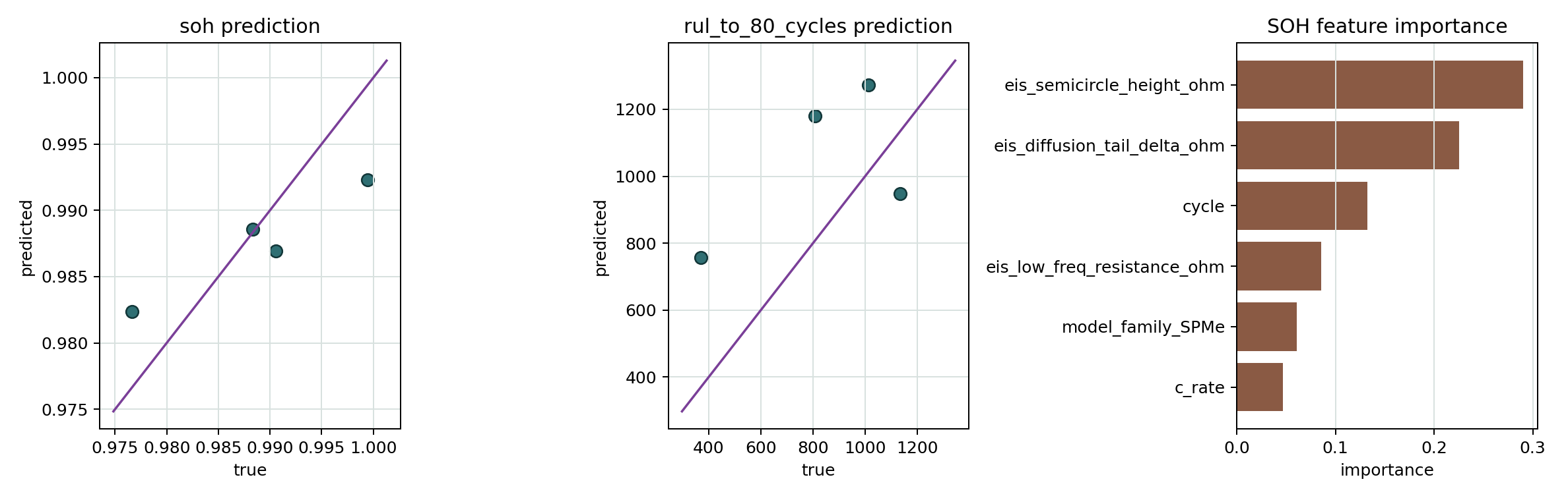
电池建模与 AI / DIAGRAM
SOH/RUL 训练结果图
展示 held-out SOH/RUL 预测散点图和 SOH 特征重要性。
电池建模与 AI / ARCHIVE
PyBaMM AI Data Lab 完整实验包
打包设计生成、老化 sweep、EIS sweep、标签构建、质量检查、样例 CSV 和图示。
项目时间线
已发布文章
- PyBaMM 快速解读:从 Oxford 电池模型架构到 AI 数据管线 面向博士生拆解 PyBaMM expression tree、Simulation 管线、模型选项和 AI 数据 schema。
- PyBaMM 阻抗谱数据生成:EISSimulation、SOC sweep 与 AI 标签 用 PyBaMM core 的 EISSimulation 生成阻抗谱,提取 Nyquist/Bode 特征并对齐老化标签。
- 用 PyBaMM 生成电池老化与阻抗 AI 数据集:标签、切分和质量控制 构建可复现 PyBaMM 数据工厂,生成 SOH、RUL、LLI、LAM、plating 和 EIS 特征标签。
- 训练电池 AI 实例:用 PyBaMM 仿真数据预测 SOH 与 RUL 用 PyBaMM 或 surrogate 生成的 EIS 特征和工况数据训练 scikit-learn 模型,预测电池 SOH 与 RUL。
已公开资源
- PyBaMM AI Data Lab 说明 说明 PyBaMM 电池建模与 AI 数据管线的安装、quick run、backend 和输出 schema。
- PyBaMM AI Data Lab 完整实验包 打包设计生成、老化 sweep、EIS sweep、标签构建、质量检查、样例 CSV 和图示。
- PyBaMM 样本 manifest 保存 sample_id、模型族、参数集、协议、温度、SOC、cycle、split group 和标签来源。
- PyBaMM EIS 样例谱 CSV 频点级阻抗输出,包含 frequency、Z_re、Z_im、幅值、相位、backend 和 solver status。
- 电池老化与阻抗标签 CSV 保存 SOH、RUL proxy、LLI、LAM、plating、local resistance 和 EIS 特征。
- PyBaMM AI 数据质量报告 记录重复 sample、频点重复、缺失标签、split leakage 和 backend 使用情况。
- PyBaMM 到 AI 数据管线图 展示设计网格、老化求解、EIS 求解、标签构建、质量门和 AI split。
- EIS 特征与标签 schema 图 把频点、阻抗特征、工况 metadata 与 SOH/RUL/退化模式标签连接起来。
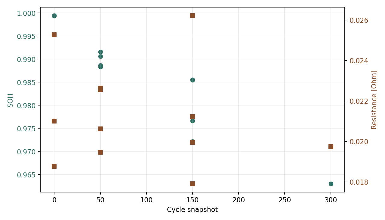
- 老化标签样例图 样例展示 cycle snapshot、SOH 与 local ECM resistance 的标签变化。
- SOH/RUL 训练指标 CSV 保存 group split、MAE、RMSE、R2、label source 和 backend used,用于复查训练结果。
- SOH/RUL held-out 预测 CSV 保存测试样本的真实值、预测值和绝对误差。
- SOH/RUL 特征重要性 CSV 记录每个目标模型的随机森林特征重要性。
- SOH/RUL 训练结果图 展示 held-out SOH/RUL 预测散点图和 SOH 特征重要性。
- 电池建模与 AI 分享图 面向 PyBaMM 电池建模、EIS、老化仿真和 AI 数据专题的 OG 分享图。
下一步计划
- 补充实验数据校准与参数可识别性笔记
- 增加 PyBOP/SEIS 对照实验的重新验证版本