
English
Training a Battery AI Model with PyBaMM: Predicting SOH and RUL
The previous architecture established the pipeline for generating physics-based Impedance (EIS) tensors via PyBaMM. We now pivot to the most heavily scrutinized step in battery informatics: training sequence-to-sequence deep learning models (LSTMs, Transformers) to predict State of Health (SOH) and Remaining Useful Life (RUL). We discard simplistic feature-engineering in favor of mapping high-dimensional electrochemical states to prognostic life trajectories.
Physics-based synthetic samples generated by rigorous DFN/SPMe formulations are invaluable for pretraining Physics-Informed Neural Networks (PINNs) and validating estimator covariance matrices, but they strictly necessitate eventual alignment with empirical cell degradation paths.
1. The Stochastic Degradation Dynamics
Battery aging is non-Markovian; the internal state at cycle $k$ depends on the entire stress history. In the context of optimal estimation theory, the SOH and RUL are treated as unobserved latent states within a discrete-time nonlinear dynamical system. A canonical representation for SOH tracking utilizes the Extended Kalman Filter (EKF) formulation:
State transition model (incorporating SEI thickening and active material loss):
$$ x_{k+1} = f(x_k, u_k) + w_k, quad w_k sim mathcal{N}(0, Q) $$
Observation model (EIS spectra and terminal voltage limits):
$$ y_k = h(x_k, u_k) + v_k, quad v_k sim mathcal{N}(0, R) $$
Where $x_k$ encapsulates the internal capacity parameters (LLI, LAM) corresponding to SOH. Our deep learning task replaces the heuristic observation function $h(cdot)$ with a differentiable neural network parameterized by $theta$, optimizing the joint log-likelihood of the degradation trajectory.
2. Deep Sequence Architectures for Prognostics
To capture the long-term temporal dependencies of capacity fade and the specific onset of the nonlinear "knee" point, we implement a Transformer encoder architecture. Unlike basic feed-forward networks, attention mechanisms natively process the variable-length cycle histories of Nyquist tensors.
import torch
import torch.nn as nn

class ImpedanceTransformer(nn.Module):
    def __init__(self, input_dim=120, d_model=256, nhead=8, num_layers=4):
        super().__init__()
        # Project raw EIS tensors (Re, Im arrays) into latent space
        self.input_projection = nn.Linear(input_dim, d_model)

        # Positional encoding for cycle number
        self.pos_encoder = PositionalEncoding(d_model)

        # Transformer Encoder processing temporal degradation
        encoder_layers = nn.TransformerEncoderLayer(d_model=d_model, nhead=nhead, batch_first=True)
        self.transformer = nn.TransformerEncoder(encoder_layers, num_layers=num_layers)

        # Multi-task head: SOH regression and RUL expectation
        self.soh_head = nn.Linear(d_model, 1)
        self.rul_head = nn.Sequential(
            nn.Linear(d_model, 64),
            nn.GELU(),
            nn.Linear(64, 1),
            nn.Softplus() # RUL is strictly positive
        )

    def forward(self, eis_sequence):
        # eis_sequence shape: [batch_size, sequence_length, input_dim]
        x = self.input_projection(eis_sequence)
        x = self.pos_encoder(x)
        features = self.transformer(x)

        # Extract features from the latest cycle for prediction
        latest_features = features[:, -1, :]
        soh_pred = self.soh_head(latest_features)
        rul_pred = self.rul_head(latest_features)

        return soh_pred, rul_pred
The input tensor comprises concatenated real and imaginary components $Z_{re}(omega)$ and $Z_{im}(omega)$ across a standardized frequency log-space, combined with operational stress factors ($T$, $Delta DOD$, $C$-rate).
3. Regularizing the Loss Surface
Predicting RUL directly is fundamentally ill-posed early in life. We structure the loss function $mathcal{L}(theta)$ using a multi-task paradigm with physics-informed regularization:
$$ mathcal{L}(theta) = lambda_1 | text{SOH}_{pred} - text{SOH}_{true} |_2^2 + lambda_2 text{Huber}(text{RUL}_{pred}, text{RUL}_{true}) + lambda_3 Phi(x) $$
Where $Phi(x)$ enforces physical monotonicity constraints (e.g., SOH strictly monotonically decreasing barring relaxation phenomena).
4. Combating Covariate Shift and Leakage
The cardinal sin in synthetic data ML is row-wise independent splitting. Time-series data derived from a singular PyBaMM Simulation.solve() trajectory exhibits deterministic covariance. If cycle $N$ and cycle $N+1$ from the same cell fall into train and test sets respectively, the Transformer trivializes the prediction task via linear interpolation, yielding a catastrophic generalization failure when deployed on hardware.
We enforce strict out-of-distribution (OOD) cross-validation by stratifying the splits across orthogonal dimensions of the parameter space using cell_design_id or protocol_id:
from sklearn.model_selection import GroupKFold

# Splitting purely by deterministic physical configurations
gkf = GroupKFold(n_splits=5)
for train_idx, test_idx in gkf.split(X, y, groups=metadata["cell_design_id"]):
    train_tensor = X[train_idx]
    # Execute PyTorch training loop
5. Deploying to BMS Microcontrollers
A real-world BMS relies on ASIL-rated MCUs computing at sub-100 MHz. The massive multi-headed attention weights developed in PyTorch must be aggressively compressed. We utilize post-training quantization (PTQ) to Int8 and structural pruning to strip 95% of the model footprint. The residual network is exported via ONNX, integrated with an embedded C++ inference engine, and deployed adjacent to the hardware EKF matrix math.
References
Chinese
训练电池 AI 实例:用 PyBaMM 仿真数据预测 SOH 与 RUL
Open as a full page前述架构已经建立了利用 PyBaMM 生成基于物理的阻抗 (EIS) 张量的完整数据流。现在我们将进入电池信息学中最核心且最受学术界审视的阶段:训练序列到序列的深度学习模型(如 LSTMs, Transformers)来预测健康状态 (SOH) 与剩余使用寿命 (RUL)。我们抛弃了简单的特征工程,转而研究将高维电化学状态直接映射到电池生命周期轨迹的方法。
由严谨的 DFN/SPMe 模型生成的基于物理的合成样本,对于预训练物理信息神经网络 (PINN) 和验证状态估计器协方差矩阵具有不可估量的价值,但在最终应用时严格需要与实际电芯退化路径进行标定对齐。
一、退化动力学的随机过程建模
电池老化是一个非马尔可夫 (non-Markovian) 过程;在循环 $k$ 时的内部状态取决于整个生命周期的应力历史。在最优估计理论的框架下,SOH 和 RUL 被视为离散时间非线性动力系统中的不可见隐状态。用于 SOH 追踪的经典表示方法通常采用扩展卡尔曼滤波 (EKF) 公式:
状态转移模型(包含 SEI 增厚与活性物质损失):
$$ x_{k+1} = f(x_k, u_k) + w_k, quad w_k sim mathcal{N}(0, Q) $$
观测模型(EIS 谱图与端电压极限):
$$ y_k = h(x_k, u_k) + v_k, quad v_k sim mathcal{N}(0, R) $$
这里,$x_k$ 封装了直接对应于 SOH 的内部容量参数(如 LLI、LAM)。我们的深度学习任务,就是用参数为 $theta$ 的可微神经网络替换掉传统的启发式观测函数 $h(cdot)$,从而最大化退化轨迹的联合对数似然。
二、用于预测预测的深度序列架构
为了捕获容量衰减的长期时序依赖性以及非线性“跳水点” (knee point) 的确切发生时机,我们实现了 Transformer 编码器架构。与基础的前馈网络不同,注意力机制天生具备处理 Nyquist 张量可变长度循环历史的能力。
import torch
import torch.nn as nn

class ImpedanceTransformer(nn.Module):
    def __init__(self, input_dim=120, d_model=256, nhead=8, num_layers=4):
        super().__init__()
        # 将原始 EIS 张量 (实部、虚部数组) 投影到隐空间
        self.input_projection = nn.Linear(input_dim, d_model)

        # 针对循环次数的位置编码
        self.pos_encoder = PositionalEncoding(d_model)

        # 处理时序退化特征的 Transformer 编码器
        encoder_layers = nn.TransformerEncoderLayer(d_model=d_model, nhead=nhead, batch_first=True)
        self.transformer = nn.TransformerEncoder(encoder_layers, num_layers=num_layers)

        # 多任务输出头:SOH 连续回归与 RUL 期望
        self.soh_head = nn.Linear(d_model, 1)
        self.rul_head = nn.Sequential(
            nn.Linear(d_model, 64),
            nn.GELU(),
            nn.Linear(64, 1),
            nn.Softplus() # RUL 必须是严格的正数
        )

    def forward(self, eis_sequence):
        # eis_sequence 维度: [batch_size, sequence_length, input_dim]
        x = self.input_projection(eis_sequence)
        x = self.pos_encoder(x)
        features = self.transformer(x)

        # 提取最新循环的特征用于最终预测
        latest_features = features[:, -1, :]
        soh_pred = self.soh_head(latest_features)
        rul_pred = self.rul_head(latest_features)

        return soh_pred, rul_pred
输入张量由标准化对数频率空间下的实部 $Z_{re}(omega)$ 和虚部 $Z_{im}(omega)$ 级联而成,并融合了操作应力因子(如温度 $T$、放电深度 $Delta DOD$、充放电倍率 $C$-rate)。
三、损失曲面的正则化
在电池寿命早期直接预测 RUL 本质上是一个不适定 (ill-posed) 问题。我们采用包含物理信息正则化的多任务范式来构建损失函数 $mathcal{L}(theta)$:
$$ mathcal{L}(theta) = lambda_1 | text{SOH}_{pred} - text{SOH}_{true} |_2^2 + lambda_2 text{Huber}(text{RUL}_{pred}, text{RUL}_{true}) + lambda_3 Phi(x) $$
其中,惩罚项 $Phi(x)$ 用于强制施加物理单调性约束(例如,排除静置恢复现象后,SOH 必须是严格单调递减的)。
四、对抗协变量偏移与数据泄漏
在合成数据机器学习中,最致命的错误就是执行逐行的独立随机拆分。从单个 PyBaMM Simulation.solve() 轨迹中派生的时间序列数据具有完全确定性的协方差。如果同一电芯的第 $N$ 次循环和第 $N+1$ 次循环分别落入训练集和测试集,Transformer 会轻易通过线性插值“作弊”完成预测任务,这将导致模型在部署到实际硬件时发生灾难性的泛化失败。
我们必须通过使用 cell_design_id 或 protocol_id 在参数空间的正交维度上对拆分进行分层,来强制执行严格的分布外 (OOD) 交叉验证:
from sklearn.model_selection import GroupKFold

# 完全依据确定性的物理配置组进行拆分
gkf = GroupKFold(n_splits=5)
for train_idx, test_idx in gkf.split(X, y, groups=metadata["cell_design_id"]):
    train_tensor = X[train_idx]
    # 执行 PyTorch 训练循环
五、向 BMS 微控制器部署的工程挑战
真实的 BMS 依赖于算力不足 100 MHz 且具备 ASIL 安全等级的车规级 MCU。在 PyTorch 中训练出的庞大且包含多头注意力权重的模型必须经过极端的压缩。我们利用训练后量化 (PTQ) 技术将其转换为 Int8 精度,并结合结构化剪枝去除了 95% 的模型体积。残余的高效网络通过 ONNX 导出,与底层的 C++ 推理引擎集成,并部署在硬件 EKF 矩阵数学运算模块旁运行。
References
The previous architecture established the pipeline for generating physics-based Impedance (EIS) tensors via PyBaMM. We now pivot to the most heavily scrutinized step in battery informatics: training sequence-to-sequence deep learning models (LSTMs, Transformers) to predict State of Health (SOH) and Remaining Useful Life (RUL). We discard simplistic feature-engineering in favor of mapping high-dimensional electrochemical states to prognostic life trajectories.
Physics-based synthetic samples generated by rigorous DFN/SPMe formulations are invaluable for pretraining Physics-Informed Neural Networks (PINNs) and validating estimator covariance matrices, but they strictly necessitate eventual alignment with empirical cell degradation paths.
1. The Stochastic Degradation Dynamics
Battery aging is non-Markovian; the internal state at cycle $k$ depends on the entire stress history. In the context of optimal estimation theory, the SOH and RUL are treated as unobserved latent states within a discrete-time nonlinear dynamical system. A canonical representation for SOH tracking utilizes the Extended Kalman Filter (EKF) formulation:
State transition model (incorporating SEI thickening and active material loss):
$$ x_{k+1} = f(x_k, u_k) + w_k, quad w_k sim mathcal{N}(0, Q) $$
Observation model (EIS spectra and terminal voltage limits):
$$ y_k = h(x_k, u_k) + v_k, quad v_k sim mathcal{N}(0, R) $$
Where $x_k$ encapsulates the internal capacity parameters (LLI, LAM) corresponding to SOH. Our deep learning task replaces the heuristic observation function $h(cdot)$ with a differentiable neural network parameterized by $theta$, optimizing the joint log-likelihood of the degradation trajectory.
2. Deep Sequence Architectures for Prognostics
To capture the long-term temporal dependencies of capacity fade and the specific onset of the nonlinear “knee” point, we implement a Transformer encoder architecture. Unlike basic feed-forward networks, attention mechanisms natively process the variable-length cycle histories of Nyquist tensors.
import torch
import torch.nn as nn

class ImpedanceTransformer(nn.Module):
    def __init__(self, input_dim=120, d_model=256, nhead=8, num_layers=4):
        super().__init__()
        # Project raw EIS tensors (Re, Im arrays) into latent space
        self.input_projection = nn.Linear(input_dim, d_model)

        # Positional encoding for cycle number
        self.pos_encoder = PositionalEncoding(d_model)

        # Transformer Encoder processing temporal degradation
        encoder_layers = nn.TransformerEncoderLayer(d_model=d_model, nhead=nhead, batch_first=True)
        self.transformer = nn.TransformerEncoder(encoder_layers, num_layers=num_layers)

        # Multi-task head: SOH regression and RUL expectation
        self.soh_head = nn.Linear(d_model, 1)
        self.rul_head = nn.Sequential(
            nn.Linear(d_model, 64),
            nn.GELU(),
            nn.Linear(64, 1),
            nn.Softplus() # RUL is strictly positive
        )

    def forward(self, eis_sequence):
        # eis_sequence shape: [batch_size, sequence_length, input_dim]
        x = self.input_projection(eis_sequence)
        x = self.pos_encoder(x)
        features = self.transformer(x)

        # Extract features from the latest cycle for prediction
        latest_features = features[:, -1, :]
        soh_pred = self.soh_head(latest_features)
        rul_pred = self.rul_head(latest_features)

        return soh_pred, rul_pred
The input tensor comprises concatenated real and imaginary components $Z_{re}(omega)$ and $Z_{im}(omega)$ across a standardized frequency log-space, combined with operational stress factors ($T$, $Delta DOD$, $C$-rate).
3. Regularizing the Loss Surface
Predicting RUL directly is fundamentally ill-posed early in life. We structure the loss function $mathcal{L}(theta)$ using a multi-task paradigm with physics-informed regularization:
$$ mathcal{L}(theta) = lambda_1 | text{SOH}_{pred} – text{SOH}_{true} |_2^2 + lambda_2 text{Huber}(text{RUL}_{pred}, text{RUL}_{true}) + lambda_3 Phi(x) $$
Where $Phi(x)$ enforces physical monotonicity constraints (e.g., SOH strictly monotonically decreasing barring relaxation phenomena).
4. Combating Covariate Shift and Leakage
The cardinal sin in synthetic data ML is row-wise independent splitting. Time-series data derived from a singular PyBaMM Simulation.solve() trajectory exhibits deterministic covariance. If cycle $N$ and cycle $N+1$ from the same cell fall into train and test sets respectively, the Transformer trivializes the prediction task via linear interpolation, yielding a catastrophic generalization failure when deployed on hardware.
We enforce strict out-of-distribution (OOD) cross-validation by stratifying the splits across orthogonal dimensions of the parameter space using cell_design_id or protocol_id:
from sklearn.model_selection import GroupKFold

# Splitting purely by deterministic physical configurations
gkf = GroupKFold(n_splits=5)
for train_idx, test_idx in gkf.split(X, y, groups=metadata["cell_design_id"]):
    train_tensor = X[train_idx]
    # Execute PyTorch training loop
5. Deploying to BMS Microcontrollers
A real-world BMS relies on ASIL-rated MCUs computing at sub-100 MHz. The massive multi-headed attention weights developed in PyTorch must be aggressively compressed. We utilize post-training quantization (PTQ) to Int8 and structural pruning to strip 95% of the model footprint. The residual network is exported via ONNX, integrated with an embedded C++ inference engine, and deployed adjacent to the hardware EKF matrix math.
References
Search questions
FAQ
Who is this article for?
This article is for readers who want a phd level-level guide to Training a Battery AI Model with PyBaMM: Predicting SOH and RUL. It takes about 14 min and focuses on PyBaMM, scikit-learn, SOH, RUL.
What should I read next?
Use the related tutorials and project links below the article to continue through the closest topic hub.
Does this article include runnable code or companion resources?
Yes. Use the run notes, resource cards, and download links on the page to reproduce the example or inspect the companion files.
How does this article fit into the larger site?
It is connected to the article context block, learning routes, resources, and project timeline so readers can move from concept to implementation.
Article context
Battery Modeling for AI
A reproducible path from PyBaMM, EIS, and aging simulation to labeled battery datasets for AI training.
Your next step
Open resourceTrain scikit-learn regressors on PyBaMM-style EIS features and operating metadata to predict battery SOH and RUL.
Download share card Open share center
Companion resources
Battery Modeling for AI / DATASET
SOH/RUL training metrics CSV
Stores group split, MAE, RMSE, R2, label source, and backend used for auditing model results.
Battery Modeling for AI / DATASET
SOH/RUL held-out predictions CSV
Stores held-out true values, predictions, and absolute errors.
Battery Modeling for AI / DATASET
SOH/RUL feature importance CSV
Records random-forest feature importance values for each target model.
Battery Modeling for AI / DIAGRAM
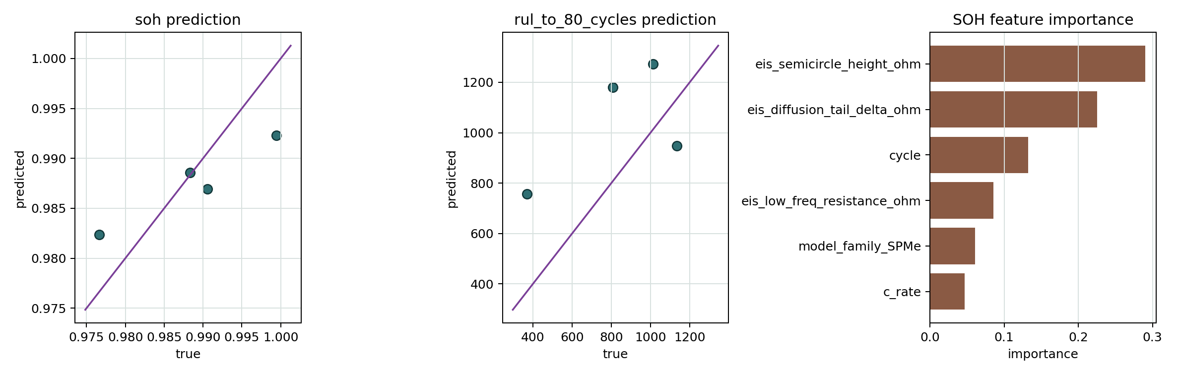
SOH/RUL training results figure
Shows held-out SOH/RUL prediction scatter plots and SOH feature importance.
Battery Modeling for AI / ARCHIVE
PyBaMM AI Data Lab full bundle
Bundles design generation, aging sweeps, EIS sweeps, label building, validation checks, sample CSVs, and figures.
Project timeline
Published posts
- Reading PyBaMM Fast: Architecture for Battery Modeling and AI Data A PhD-level guide to PyBaMM expression trees, Simulation, model options, metadata, and AI dataset design.
- PyBaMM EIS Data Generation: Impedance Features and AI Labels Use PyBaMM core EISSimulation to generate impedance spectra, extract features, and align them with aging labels.
- Generate Battery Aging and EIS AI Datasets with PyBaMM Build a reproducible PyBaMM data factory for SOH, RUL, LLI, LAM, plating, and impedance-feature labels.
- Training a Battery AI Model with PyBaMM: Predicting SOH and RUL Train scikit-learn regressors on PyBaMM-style EIS features and operating metadata to predict battery SOH and RUL.
Published resources
- PyBaMM AI Data Lab README Setup, quick run, backend behavior, and output schemas for the PyBaMM battery AI data pipeline.
- PyBaMM AI Data Lab full bundle Bundles design generation, aging sweeps, EIS sweeps, label building, validation checks, sample CSVs, and figures.
- PyBaMM sample manifest Stores sample id, model family, parameter set, protocol, temperature, SOC, cycle, split group, and label source.
- PyBaMM EIS sample spectra CSV Frequency-level impedance output with frequency, Z_re, Z_im, magnitude, phase, backend, and solver status.
- Battery aging and EIS labels CSV Stores SOH, RUL proxy, LLI, LAM, plating, local resistance, and EIS features.
- PyBaMM AI data quality report Records duplicate samples, duplicate spectrum points, missing labels, split leakage, and backend usage.
- PyBaMM to AI data pipeline figure Shows design grid, aging solve, EIS solve, label build, quality gate, and AI split.
- EIS feature and label schema figure Connects frequency points, impedance features, operating metadata, and SOH/RUL/degradation labels.
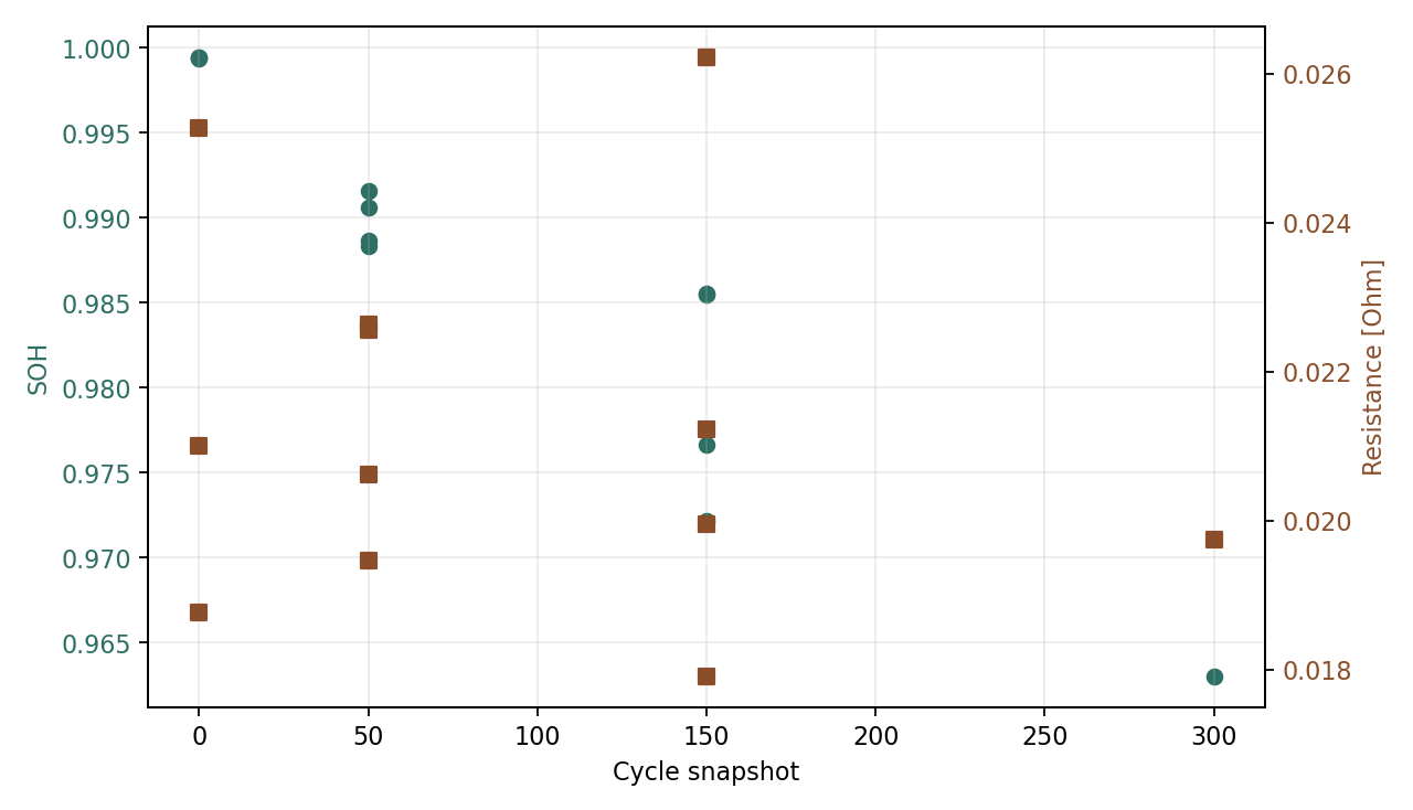
- Aging label sample figure Sample figure showing cycle snapshots, SOH, and local ECM resistance labels.
- SOH/RUL training metrics CSV Stores group split, MAE, RMSE, R2, label source, and backend used for auditing model results.
- SOH/RUL held-out predictions CSV Stores held-out true values, predictions, and absolute errors.
- SOH/RUL feature importance CSV Records random-forest feature importance values for each target model.
- SOH/RUL training results figure Shows held-out SOH/RUL prediction scatter plots and SOH feature importance.
- Battery Modeling for AI share card OG share card for the PyBaMM battery modeling, EIS, aging simulation, and AI data hub.
Next notes
- Add experimental calibration and identifiability notes
- Add revalidated PyBOP/SEIS comparison notes