
English
Reading PyBaMM Fast: Architecture for Battery Modeling and AI Data
This article is strictly intended for PhD-level computational electrochemists, numerical modelers, and machine learning researchers whose work demands rigorous, physics-informed architectures. The goal is not merely to run PyBaMM as an opaque impedance simulator, but to dissect its underlying directed acyclic graph (DAG) symbolic architecture: how sets of partial differential equations (PDEs) are parsed into expression trees, how parameters are mapped into these graphs, how differential-algebraic equations (DAEs) are passed to stiff solvers like CasADi and SUNDIALS, and how the resulting state variables are rigorously formulated as labels for AI datasets.
For those searching for “PyBAMM”, the official project name is PyBaMM (Python Battery Mathematical Modelling). Modern Electrochemical Impedance Spectroscopy (EIS) workflows should bypass legacy wrappers and interface directly with the core pybamm.EISSimulation object, which linearizes the underlying DAE system in the frequency domain.

1. PyBaMM as a Differential-Algebraic Equation Compiler Pipeline
The architectural genius of the PyBaMM framework lies in its abstraction of electrochemical physics into a symbolic expression tree before any numerical discretization occurs. In practice, the Simulation class acts as an advanced compiler front-end. It translates continuum mechanics and electrochemical PDEs into a discretized state-space format.
When engineering within the PyBaMM source code, one must navigate the pipeline in this specific order of instantiation:
- Model Formulation: Single Particle Model (SPM), SPM with electrolyte (SPMe), or the Doyle-Fuller-Newman (DFN) pseudo-two-dimensional (P2D) porous electrode model.
- Submodel Options: Activating localized physical phenomena such as Solid Electrolyte Interphase (SEI) growth kinetics, lithium plating overpotentials, particle fracture mechanics, Loss of Active Material (LAM), and specific surface area formulations.
- Parameterization: Injecting highly non-linear functions (e.g., OCP curves) and scalar properties mapping abstract symbols to physical quantities.
- Experiment / Protocol: Defining current density inputs, cut-off voltages, CCCV cycling, and boundary conditions.
- Discretization and Solver: Spatial discretizations (Finite Volume Method) converting PDEs to DAEs, fed into backwards differentiation formula (BDF) solvers capable of handling extreme stiffness.
2. The Mathematical Rigor of the DFN Model
To appreciate the underlying solver complexity, we must formalize the physics. The DFN model solves coupled conservation laws across solid and electrolyte phases. The solid-phase lithium concentration $c_s(r,x,t)$ within active material particles is governed by Fick's Second Law in spherical coordinates:
$$ frac{partial c_s}{partial t} = frac{1}{r^2} frac{partial}{partial r} left( r^2 D_s(c_s) frac{partial c_s}{partial r} right) $$
This is coupled to the electrochemical reaction at the particle-electrolyte interface via the Butler-Volmer kinetic equation, which dictates the volumetric transfer current density $j(x,t)$:
$$ j = a_s i_0 left[ expleft(frac{alpha_a F eta}{R T}right) - expleft(-frac{alpha_c F eta}{R T}right) right] $$
Where the exchange current density $i_0$ depends on $c_s$, $c_e$ (electrolyte concentration), and the local activation overpotential $eta = phi_s - phi_e - U_{OCP}(c_s)$. The resulting highly coupled, non-linear PDE system exhibits severe stiffness, especially when boundary layers form at high C-rates.
3. Symbolic Math Trees and Automatic Differentiation
PyBaMM avoids hard-coding sparse matrices. Instead, equations like the diffusion PDE are constructed using symbolic nodes (e.g., pybamm.Variable, pybamm.Gradient, pybamm.Divergence). Consider this minimal syntax for defining a solid-phase diffusion operator:
import pybamm

# Symbolic definition of concentration and diffusion coefficient
c_s = pybamm.Variable("Solid concentration")
D_s = pybamm.Parameter("Solid diffusion coefficient")

# Fick's Second Law as a symbolic expression tree
N_s = -D_s * pybamm.grad(c_s)  # Flux
dcdt = -pybamm.div(N_s)        # Rate of change

# The tree structure enables automatic differentiation
jacobian_node = dcdt.diff(c_s)
This symbolic graph is critical. It allows PyBaMM to seamlessly substitute parameter sets, discretize over arbitrary meshes, and—most importantly—leverage Automatic Differentiation (AD) via CasADi. Constructing exact, dense analytical Jacobians analytically reduces the Newton iterations required by implicit solvers during time-stepping.
4. Numerical Engineering: CasADi and SUNDIALS for Stiff DAEs
Once spatially discretized, the DFN model yields a massive system of stiff Ordinary Differential Equations (ODEs) and Algebraic Equations. The characteristic time constants range from microseconds (double-layer capacitance) to hours (solid diffusion). Explicit methods (like Runge-Kutta 4) will fail spectacularly due to the CFL condition.
PyBaMM addresses this by compiling the symbolic tree into CasADi SX/MX graph objects. CasADi generates highly optimized C-code for the right-hand-side evaluations and Jacobians. This is handed off to SUNDIALS (specifically the IDA/IDAS or CVODES solver packages), which implements Variable-Order Variable-Step BDF methods. The solver adapts its step size dynamically, taking nano-second steps during current transients and minute-long steps during rest periods.
5. Physical Fidelity vs. Sample Count in AI Pipelines
For machine learning researchers, understanding the origin of your synthetic data is paramount. SPM, SPMe, and DFN are not just accuracy tiers; they represent completely different state spaces.
- SPM (Single Particle Model): Assumes infinite electrolyte conductivity and uniform electrolyte concentration. Suitable for representing macroscopic State of Health (SOH) and simple RUL forecasting where electrolyte dynamics do not limit the cell.
- SPMe (SPM with electrolyte): Reintroduces analytical approximations of electrolyte concentration gradients.
- DFN (Doyle-Fuller-Newman): Resolves exact spatial profiles across anode, separator, and cathode. Absolutely mandatory for generating AI data targeting high-rate polarization, localized lithium plating, and precise frequency-dependent EIS arcs where solid-liquid coupling dominates.
6. Minimum AI Sample Schema
A rigorous dataset must be structured for falsifiability. An auditable training row should include:
- Boundary Conditions: Initial $c_s$ distribution (SOC), operational temperature, C-rate limits, and exact frequency excitation grid.
- Observational Variables: Terminal voltage statistics, real ($Z_{re}$) and imaginary ($Z_{im}$) impedance components, high-frequency intercept, and Warburg diffusion tail coefficients.
- Physics-Informed Labels: Explicit tracking of LLI (moles of Li lost to SEI), LAM (volume fraction of fractured particles), and localized ECM equivalent parameters.
7. Common Methodological Pitfalls
- Treating simulations as experimental ground truth. Synthetic data generated from DFN is a projection of a specific mathematical theory. It must be rigorously calibrated using non-linear least squares against actual cycler data.
- Maximizing permutations without physical diversity. Generating 10,000 near-identical curves through naive Monte Carlo parameter sampling causes severe manifold collapse. Focus on Latin Hypercube Sampling across physically orthogonal parameter dimensions.
- Ignoring solver tolerances. When extracting impedance features from highly degraded battery states, poor absolute/relative tolerances in SUNDIALS will inject numerical noise indistinguishable from electrochemical phenomena.
References
Chinese
PyBaMM 快速解读:从 Oxford 电池模型架构到 AI 数据管线
Open as a full page这篇文章专为具有计算电化学、数值建模和机器学习背景的博士级研究人员撰写。这些领域的工作需要极度严谨的物理信息架构。我们的目标绝不是将 PyBaMM 当作一个黑盒阻抗模拟器来运行,而是要解剖其底层的有向无环图 (DAG) 符号架构:偏微分方程组 (PDE) 如何被解析为表达式树,参数如何映射到这些图中,微分代数方程 (DAE) 如何传递给 CasADi 和 SUNDIALS 等刚性求解器,以及产生的状态变量如何被严格地构造为 AI 数据集的标签。
如果你在搜索“PyBAMM”,它的官方正式名称是 PyBaMM (Python Battery Mathematical Modelling)。现代电化学阻抗谱 (EIS) 工作流应该绕过旧版的包装器,直接与核心的 pybamm.EISSimulation 对象交互,该对象能在频域内对底层的 DAE 系统进行线性化处理。
一、将 PyBaMM 视作微分代数方程 (DAE) 的编译管线
PyBaMM 框架最核心的架构天才之处在于,它在进行任何数值离散化之前,先将电化学物理过程抽象为一个符号表达式树 (symbolic expression tree)。在实际操作中,Simulation 类扮演着高级编译器前端的角色。它将连续介质力学和电化学 PDE 转化为离散化的状态空间格式。
在深入 PyBaMM 源码进行工程开发时,必须按照以下特定的实例化顺序来梳理逻辑:
- 模型构建 (Model):选择单颗粒模型 (SPM)、含电解液的单颗粒模型 (SPMe),或是基于准二维 (P2D) 多孔电极理论的 Doyle-Fuller-Newman (DFN) 模型。
- 子模型选项 (Options):激活局部的物理化学现象,例如固体电解质界面膜 (SEI) 生长动力学、析锂过电势、颗粒破裂力学、活性物质损失 (LAM) 以及特定的表面积公式。
- 参数化 (Parameterization):注入高度非线性的函数(如 OCP 曲线)和标量属性,将抽象符号映射为具体的物理量。
- 实验协议 (Experiment):定义电流密度输入、截止电压、CCCV 循环工况和各种边界条件。
- 离散化与求解器 (Discretization and Solver):使用有限体积法 (FVM) 进行空间离散化,将 PDE 转换为 DAE,然后送入能够处理极端刚性 (stiffness) 问题的后向微分公式 (BDF) 求解器。
二、DFN 模型的数学严谨性与刚性系统
为了理解底层求解器的复杂性,我们必须对物理过程进行形式化。DFN 模型求解固相和电解液相耦合的守恒定律。活性物质颗粒内部的固相锂离子浓度 $c_s(r,x,t)$ 在球坐标下受菲克第二定律 (Fick's Second Law) 支配:
$$ frac{partial c_s}{partial t} = frac{1}{r^2} frac{partial}{partial r} left( r^2 D_s(c_s) frac{partial c_s}{partial r} right) $$
这通过 Butler-Volmer 动力学方程与颗粒-电解液界面的电化学反应耦合,该方程决定了体积转移电流密度 $j(x,t)$:
$$ j = a_s i_0 left[ expleft(frac{alpha_a F eta}{R T}right) - expleft(-frac{alpha_c F eta}{R T}right) right] $$
其中交换电流密度 $i_0$ 依赖于 $c_s$、电解液浓度 $c_e$ 以及局部活化过电势 $eta = phi_s - phi_e - U_{OCP}(c_s)$。这种高度耦合、非线性的 PDE 系统表现出极强的数学刚性,特别是在高倍率 (C-rate) 放电导致边界层形成时。
三、符号数学树与自动微分 (Automatic Differentiation)
PyBaMM 彻底摒弃了硬编码稀疏矩阵的做法。相反,它使用符号节点(如 pybamm.Variable、pybamm.Gradient、pybamm.Divergence)来构造扩散 PDE 等方程。考虑以下定义固相扩散算子的核心语法片段:
import pybamm

# 符号化定义浓度和扩散系数
c_s = pybamm.Variable("Solid concentration")
D_s = pybamm.Parameter("Solid diffusion coefficient")

# 将菲克第二定律构建为符号表达式树
N_s = -D_s * pybamm.grad(c_s)  # 扩散通量 (Flux)
dcdt = -pybamm.div(N_s)        # 浓度随时间变化率

# 符号树结构使得自动微分成为可能,直接计算雅可比矩阵
jacobian_node = dcdt.diff(c_s)
这个符号图至关重要。它允许 PyBaMM 无缝地替换参数集、在任意网格上离散化,并且——最重要的是——利用 CasADi 实现自动微分 (AD)。解析地构建极其精确、稠密的分析雅可比矩阵,极大地减少了隐式求解器在时间步进过程中所需的牛顿迭代次数。
四、数值工程:用于刚性 DAE 的 CasADi 与 SUNDIALS
完成空间离散化后,DFN 模型会产生一个极其庞大且刚性极强的常微分方程 (ODE) 和代数方程系统。其特征时间常数跨度极大,从微秒级(双电层电容)到数小时级(固相扩散)。由于柯朗-弗里德里希斯-列维条件 (CFL condition) 的限制,显式方法(如四阶龙格-库塔法 RK4)在求解时将彻底崩溃。
PyBaMM 的解决方案是将符号树编译为 CasADi 的 SX/MX 计算图对象。CasADi 生成高度优化的 C 代码来评估右端项和雅可比矩阵。接着这些计算任务被移交给 SUNDIALS(特别是其中的 IDA/IDAS 或 CVODES 求解器包),这些包实现了变阶变步长的 BDF 方法。求解器动态自适应地调整步长,在电流阶跃瞬间采用纳秒级步长,而在静置阶段则可能采用长达数分钟的步长。
五、在 AI 数据管线中区分物理保真度与样本数量
对于机器学习研究者来说,理解合成数据的物理本源是重中之重。SPM、SPMe 和 DFN 不仅仅是精度上的差异,它们代表了截然不同的状态空间流形。
- SPM (单颗粒模型):假设电解液电导率无穷大且浓度均匀。只适用于描述宏观的健康状态 (SOH) 或简单的剩余使用寿命 (RUL) 预测,前提是电解液动力学不是电池的限制因素。
- SPMe (含电解液效应的单颗粒模型):重新引入了电解液浓度梯度的解析近似。
- DFN (Doyle-Fuller-Newman 模型):解析了负极、隔膜和正极的精确空间分布。如果你的 AI 数据目标是预测高倍率极化、局部析锂或精确的依赖频域的 EIS 弧段(此时固液耦合占据主导),DFN 模型是绝对不可或缺的。
六、AI 样本的严谨 Schema 设计
一个严谨的数据集必须为可证伪性 (falsifiability) 而设计。一条具备审计价值的训练样本行应当包含:
- 边界与初始条件:初始 $c_s$ 分布 (SOC)、运行温度场、充放电倍率限制以及精确的频率激励网格。
- 观测特征变量:终端电压统计量、阻抗的实部 ($Z_{re}$) 和虚部 ($Z_{im}$)、高频截距和 Warburg 扩散尾系数。
- 内嵌物理标签:显式记录由于 SEI 导致消耗的锂摩尔数 (LLI)、因颗粒破裂导致的活性物质体积分数损失 (LAM) 以及局部等效电路模型 (ECM) 参数。
七、需要避免的方法论陷阱
- 将仿真数据等同于实验真实值 (Ground Truth)。 基于 DFN 模型生成的合成数据仅仅是特定数学理论的投影。必须利用非线性最小二乘法将其与真实的充放电测试设备数据进行严格校准。
- 单纯追求样本数量而忽视物理多样性。 通过朴素的蒙特卡洛参数采样生成 10,000 条几乎相同的曲线,会导致严重的数据流形坍缩 (manifold collapse)。应该专注于在正交的物理参数维度上使用拉丁超立方采样 (LHS)。
- 忽视求解器容差设置。 当从高度退化的电池状态中提取阻抗特征时,如果 SUNDIALS 中的绝对/相对容差设置不当,将引入无法与电化学现象区分的数值噪声。
References
This article is strictly intended for PhD-level computational electrochemists, numerical modelers, and machine learning researchers whose work demands rigorous, physics-informed architectures. The goal is not merely to run PyBaMM as an opaque impedance simulator, but to dissect its underlying directed acyclic graph (DAG) symbolic architecture: how sets of partial differential equations (PDEs) are parsed into expression trees, how parameters are mapped into these graphs, how differential-algebraic equations (DAEs) are passed to stiff solvers like CasADi and SUNDIALS, and how the resulting state variables are rigorously formulated as labels for AI datasets.
For those searching for “PyBAMM”, the official project name is PyBaMM (Python Battery Mathematical Modelling). Modern Electrochemical Impedance Spectroscopy (EIS) workflows should bypass legacy wrappers and interface directly with the core pybamm.EISSimulation object, which linearizes the underlying DAE system in the frequency domain.
1. PyBaMM as a Differential-Algebraic Equation Compiler Pipeline
The architectural genius of the PyBaMM framework lies in its abstraction of electrochemical physics into a symbolic expression tree before any numerical discretization occurs. In practice, the Simulation class acts as an advanced compiler front-end. It translates continuum mechanics and electrochemical PDEs into a discretized state-space format.
When engineering within the PyBaMM source code, one must navigate the pipeline in this specific order of instantiation:
- Model Formulation: Single Particle Model (SPM), SPM with electrolyte (SPMe), or the Doyle-Fuller-Newman (DFN) pseudo-two-dimensional (P2D) porous electrode model.
- Submodel Options: Activating localized physical phenomena such as Solid Electrolyte Interphase (SEI) growth kinetics, lithium plating overpotentials, particle fracture mechanics, Loss of Active Material (LAM), and specific surface area formulations.
- Parameterization: Injecting highly non-linear functions (e.g., OCP curves) and scalar properties mapping abstract symbols to physical quantities.
- Experiment / Protocol: Defining current density inputs, cut-off voltages, CCCV cycling, and boundary conditions.
- Discretization and Solver: Spatial discretizations (Finite Volume Method) converting PDEs to DAEs, fed into backwards differentiation formula (BDF) solvers capable of handling extreme stiffness.
2. The Mathematical Rigor of the DFN Model
To appreciate the underlying solver complexity, we must formalize the physics. The DFN model solves coupled conservation laws across solid and electrolyte phases. The solid-phase lithium concentration $c_s(r,x,t)$ within active material particles is governed by Fick’s Second Law in spherical coordinates:
$$ frac{partial c_s}{partial t} = frac{1}{r^2} frac{partial}{partial r} left( r^2 D_s(c_s) frac{partial c_s}{partial r} right) $$
This is coupled to the electrochemical reaction at the particle-electrolyte interface via the Butler-Volmer kinetic equation, which dictates the volumetric transfer current density $j(x,t)$:
$$ j = a_s i_0 left[ expleft(frac{alpha_a F eta}{R T}right) – expleft(-frac{alpha_c F eta}{R T}right) right] $$
Where the exchange current density $i_0$ depends on $c_s$, $c_e$ (electrolyte concentration), and the local activation overpotential $eta = phi_s – phi_e – U_{OCP}(c_s)$. The resulting highly coupled, non-linear PDE system exhibits severe stiffness, especially when boundary layers form at high C-rates.
3. Symbolic Math Trees and Automatic Differentiation
PyBaMM avoids hard-coding sparse matrices. Instead, equations like the diffusion PDE are constructed using symbolic nodes (e.g., pybamm.Variable, pybamm.Gradient, pybamm.Divergence). Consider this minimal syntax for defining a solid-phase diffusion operator:
import pybamm

# Symbolic definition of concentration and diffusion coefficient
c_s = pybamm.Variable("Solid concentration")
D_s = pybamm.Parameter("Solid diffusion coefficient")

# Fick's Second Law as a symbolic expression tree
N_s = -D_s * pybamm.grad(c_s)  # Flux
dcdt = -pybamm.div(N_s)        # Rate of change

# The tree structure enables automatic differentiation
jacobian_node = dcdt.diff(c_s)
This symbolic graph is critical. It allows PyBaMM to seamlessly substitute parameter sets, discretize over arbitrary meshes, and—most importantly—leverage Automatic Differentiation (AD) via CasADi. Constructing exact, dense analytical Jacobians analytically reduces the Newton iterations required by implicit solvers during time-stepping.
4. Numerical Engineering: CasADi and SUNDIALS for Stiff DAEs
Once spatially discretized, the DFN model yields a massive system of stiff Ordinary Differential Equations (ODEs) and Algebraic Equations. The characteristic time constants range from microseconds (double-layer capacitance) to hours (solid diffusion). Explicit methods (like Runge-Kutta 4) will fail spectacularly due to the CFL condition.
PyBaMM addresses this by compiling the symbolic tree into CasADi SX/MX graph objects. CasADi generates highly optimized C-code for the right-hand-side evaluations and Jacobians. This is handed off to SUNDIALS (specifically the IDA/IDAS or CVODES solver packages), which implements Variable-Order Variable-Step BDF methods. The solver adapts its step size dynamically, taking nano-second steps during current transients and minute-long steps during rest periods.
5. Physical Fidelity vs. Sample Count in AI Pipelines
For machine learning researchers, understanding the origin of your synthetic data is paramount. SPM, SPMe, and DFN are not just accuracy tiers; they represent completely different state spaces.
- SPM (Single Particle Model): Assumes infinite electrolyte conductivity and uniform electrolyte concentration. Suitable for representing macroscopic State of Health (SOH) and simple RUL forecasting where electrolyte dynamics do not limit the cell.
- SPMe (SPM with electrolyte): Reintroduces analytical approximations of electrolyte concentration gradients.
- DFN (Doyle-Fuller-Newman): Resolves exact spatial profiles across anode, separator, and cathode. Absolutely mandatory for generating AI data targeting high-rate polarization, localized lithium plating, and precise frequency-dependent EIS arcs where solid-liquid coupling dominates.
6. Minimum AI Sample Schema
A rigorous dataset must be structured for falsifiability. An auditable training row should include:
- Boundary Conditions: Initial $c_s$ distribution (SOC), operational temperature, C-rate limits, and exact frequency excitation grid.
- Observational Variables: Terminal voltage statistics, real ($Z_{re}$) and imaginary ($Z_{im}$) impedance components, high-frequency intercept, and Warburg diffusion tail coefficients.
- Physics-Informed Labels: Explicit tracking of LLI (moles of Li lost to SEI), LAM (volume fraction of fractured particles), and localized ECM equivalent parameters.
7. Common Methodological Pitfalls
- Treating simulations as experimental ground truth. Synthetic data generated from DFN is a projection of a specific mathematical theory. It must be rigorously calibrated using non-linear least squares against actual cycler data.
- Maximizing permutations without physical diversity. Generating 10,000 near-identical curves through naive Monte Carlo parameter sampling causes severe manifold collapse. Focus on Latin Hypercube Sampling across physically orthogonal parameter dimensions.
- Ignoring solver tolerances. When extracting impedance features from highly degraded battery states, poor absolute/relative tolerances in SUNDIALS will inject numerical noise indistinguishable from electrochemical phenomena.
References
Search questions
FAQ
Who is this article for?
This article is for readers who want a phd level-level guide to Reading PyBaMM Fast: Architecture for Battery Modeling and AI Data. It takes about 14 min and focuses on PyBaMM, DFN, Expression Tree, AI Dataset.
What should I read next?
The recommended next step is PyBaMM EIS Data Generation: Impedance Features and AI Labels, so the article connects into a longer learning route instead of ending as an isolated note.
Does this article include runnable code or companion resources?
Yes. Use the run notes, resource cards, and download links on the page to reproduce the example or inspect the companion files.
How does this article fit into the larger site?
It is connected to the article context block, learning routes, resources, and project timeline so readers can move from concept to implementation.
Article context
Battery Modeling for AI
A reproducible path from PyBaMM, EIS, and aging simulation to labeled battery datasets for AI training.
A PhD-level guide to PyBaMM expression trees, Simulation, model options, metadata, and AI dataset design.
Download share card Open share center
Companion resources
Battery Modeling for AI / GUIDE
PyBaMM AI Data Lab README
Setup, quick run, backend behavior, and output schemas for the PyBaMM battery AI data pipeline.
Battery Modeling for AI / DIAGRAM
PyBaMM to AI data pipeline figure
Shows design grid, aging solve, EIS solve, label build, quality gate, and AI split.
Battery Modeling for AI / ARCHIVE
PyBaMM AI Data Lab full bundle
Bundles design generation, aging sweeps, EIS sweeps, label building, validation checks, sample CSVs, and figures.
Project timeline
Published posts
- Reading PyBaMM Fast: Architecture for Battery Modeling and AI Data A PhD-level guide to PyBaMM expression trees, Simulation, model options, metadata, and AI dataset design.
- PyBaMM EIS Data Generation: Impedance Features and AI Labels Use PyBaMM core EISSimulation to generate impedance spectra, extract features, and align them with aging labels.
- Generate Battery Aging and EIS AI Datasets with PyBaMM Build a reproducible PyBaMM data factory for SOH, RUL, LLI, LAM, plating, and impedance-feature labels.
- Training a Battery AI Model with PyBaMM: Predicting SOH and RUL Train scikit-learn regressors on PyBaMM-style EIS features and operating metadata to predict battery SOH and RUL.
Published resources
- PyBaMM AI Data Lab README Setup, quick run, backend behavior, and output schemas for the PyBaMM battery AI data pipeline.
- PyBaMM AI Data Lab full bundle Bundles design generation, aging sweeps, EIS sweeps, label building, validation checks, sample CSVs, and figures.
- PyBaMM sample manifest Stores sample id, model family, parameter set, protocol, temperature, SOC, cycle, split group, and label source.
- PyBaMM EIS sample spectra CSV Frequency-level impedance output with frequency, Z_re, Z_im, magnitude, phase, backend, and solver status.
- Battery aging and EIS labels CSV Stores SOH, RUL proxy, LLI, LAM, plating, local resistance, and EIS features.
- PyBaMM AI data quality report Records duplicate samples, duplicate spectrum points, missing labels, split leakage, and backend usage.
- PyBaMM to AI data pipeline figure Shows design grid, aging solve, EIS solve, label build, quality gate, and AI split.
- EIS feature and label schema figure Connects frequency points, impedance features, operating metadata, and SOH/RUL/degradation labels.
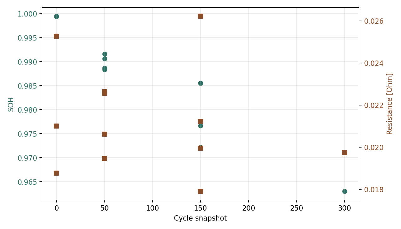
- Aging label sample figure Sample figure showing cycle snapshots, SOH, and local ECM resistance labels.
- SOH/RUL training metrics CSV Stores group split, MAE, RMSE, R2, label source, and backend used for auditing model results.
- SOH/RUL held-out predictions CSV Stores held-out true values, predictions, and absolute errors.
- SOH/RUL feature importance CSV Records random-forest feature importance values for each target model.
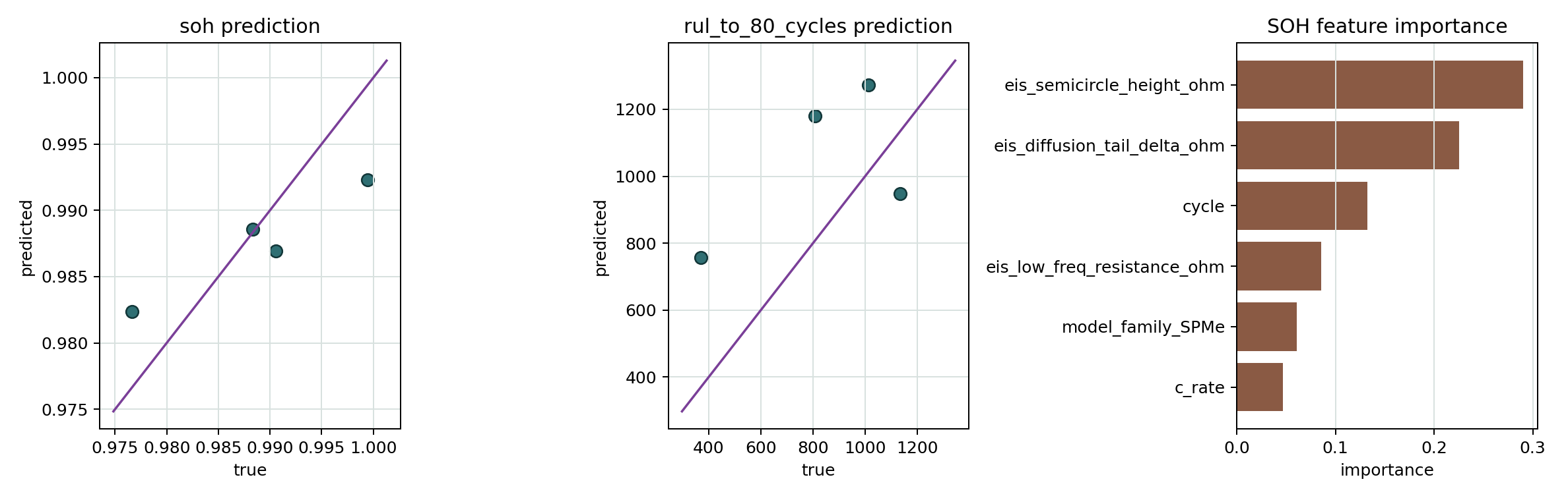
- SOH/RUL training results figure Shows held-out SOH/RUL prediction scatter plots and SOH feature importance.
- Battery Modeling for AI share card OG share card for the PyBaMM battery modeling, EIS, aging simulation, and AI data hub.
Next notes
- Add experimental calibration and identifiability notes
- Add revalidated PyBOP/SEIS comparison notes