
English
Generate Battery Aging and EIS AI Datasets with PyBaMM
Generating massive, properly labeled battery datasets using PyBaMM transcends simple computational for-loops; it is an intensive problem of numerical design of experiments (DoE). To generate data that truly empowers AI models without teaching them simulator-induced artifacts, one must rigorously control the physical boundary value problem, parameter space topology, temperature gradients, electrochemical state vector snapshots, frequency-domain impedance grids, and the algebraic solver tolerances.
The companion lab provides a foundational implementation. However, scaling this requires deploying batch processes with high --samples settings. Keep in mind: these outputs represent deterministic solutions to systems of partial differential equations (PDEs)—they are strictly physics-based synthetic data, and must undergo non-linear least squares parameter identification to match real-world battery behavior.
1. The Formalized Dataset Objective
A mathematically rigorous AI battery dataset is a collection of tuples:
$$ mathcal{D} = {(mathbf{x}_i, mathbf{y}_i, mathbf{m}_i)}_{i=1}^N $$
Here, $mathbf{x}_i in mathbb{R}^p$ represents the observable feature vector (time-series voltage transients, complex impedance $Z(omega)$, operational protocols). The target vector $mathbf{y}_i in mathbb{R}^q$ represents internal unobservables (SOH, Loss of Lithium Inventory [LLI], Loss of Active Material [LAM]). Crucially, $mathbf{m}_i$ is the exact metadata graph encapsulating the structural model assumptions, thermodynamic parameters, and solver configuration. Without $mathbf{m}_i$, the physical causality of the mapping $f: mathbf{x} rightarrow mathbf{y}$ is undefined.
2. Degradation Kinetics and State Labels
When extracting labels, we are actually querying the integrated state of specific degradation PDEs. For example, the rate of Solid Electrolyte Interphase (SEI) thickness $L_{SEI}$ growth, which drives LLI, is often modeled via solvent reduction kinetics:
$$ frac{partial L_{SEI}}{partial t} = frac{M_{SEI}}{rho_{SEI} z F} j_{SEI} expleft( -frac{E_a}{R T} right) expleft( -frac{alpha F (phi_s - phi_e - U_{SEI})}{R T} right) $$
- SOH: Defined as the integrated discharge capacity over the nominal capacity $Q_k / Q_0$.
- RUL-to-80: The projected cyclic horizon until the manifold intersects $SOH = 0.8$.
- LLI: The cumulative integral of parasitic side reaction currents.
- LAM: Often governed by particle fracture mechanics, driven by the stress tensor $sigma_{t, max}$ exceeding the material's yield strength.
- EIS Vectors: Generated via perturbation and linearization of the full DFN Jacobian in the frequency domain, capturing charge-transfer semi-circles and Warburg diffusion tails.
3. Non-Linear Least Squares Parameter Identification
Before synthetic data can be trusted, the underlying parameter distributions must be fitted to experimental data. This is typically achieved by minimizing an objective function $J(mathbf{p})$ representing the sum of squared residuals between experimental voltage $V_{exp}$ and the PyBaMM simulated voltage $V_{sim}(mathbf{p})$, utilizing optimizers like L-BFGS-B or Nelder-Mead (e.g., via PyBOP or SciPy).
import pybamm
import numpy as np
import scipy.optimize as opt

def objective(params_array):
    # Map array to PyBaMM parameters
    parameter_values.update({
        "Negative electrode active material volume fraction": params_array[0],
        "Positive electrode active material volume fraction": params_array[1]
    })
    sim = pybamm.Simulation(model, parameter_values=parameter_values)
    sim.solve(t_eval)
    V_sim = sim.solution["Terminal voltage [V]"].entries
    # Calculate Sum of Squared Errors
    return np.sum((V_exp - V_sim)**2)

# Minimize using Sequential Least Squares Programming
res = opt.minimize(objective, initial_guess, method='SLSQP', bounds=param_bounds)
Without enforcing these physical parameter constraints through optimization, an AI model trained on the dataset will merely learn the arbitrary distribution of the Latin Hypercube Sampling rather than true electrochemistry.
4. Dataset Generation Pipeline Execution
The rigorous generation of these DAE solutions requires careful management of parallel workers to handle solver failures caused by extreme parameter combinations leading to non-convergent Jacobians.
cd pybamm-ai-data-lab
python3 -m venv .venv
source .venv/bin/activate
pip install -r requirements.txt

# Execute generating 200 high-fidelity samples utilizing CasADi solvers
python src/run_all.py --samples 200 --workers 4 --seed 7 --backend pybamm --output /tmp/pybamm-ai-dataset
5. Orthogonal Splitting and Information Leakage
If cycle snapshots from the same modeled aging trajectory (e.g., cycle 10, 50, 100 of identical cell parameters) are arbitrarily partitioned into train and test sets, the AI model will overfit to the deterministic nature of the ODEs. It will simply memorize the trajectory rather than learning the generalized degradation function.
- Perform splits strictly along orthogonal boundaries:
cell_design_idor randomized subsets of the kinetic parameter space. - Frequency-domain EIS points are structurally correlated via the Kramers-Kronig relations; adjacent frequencies from a single impedance sweep must never straddle the train/test boundary.
6. Connecting Synthetic Distributions to Real-World Physics
Synthetic generation is incredibly powerful for pre-training neural networks, testing active-learning acquisition functions, and performing ablation studies on network architectures. However, bridging the sim-to-real gap necessitates:
- Continuous calibration of the underlying PyBaMM model to Differential Voltage Analysis (DVA) and Incremental Capacity Analysis (ICA) from physical cyclers.
- Global sensitivity analysis (e.g., Sobol indices) to quantify which unobservable parameters actually influence the generated voltage features.
- Strict documentation of the solver constraints—if the SUNDIALS CVODES solver fails to meet absolute tolerances of $10^{-6}$ during severe degradation steps, those data points must be flagged as non-physical rather than fed blindly to the AI.
References
Chinese
用 PyBaMM 生成电池老化与阻抗 AI 数据集:标签、切分和质量控制
Open as a full page使用 PyBaMM 生成“海量、带物理标签”的电池数据集,其技术难度早已超越了简单的计算循环 (for-loop);它本质上是一个高度复杂的数值实验设计 (DoE) 优化问题。为了确保生成的数据能够真正赋能 AI 模型,而不是让神经网络仅仅学习到仿真器本身的数值偏差和伪像,你必须严格控制物理边值问题、参数空间的拓扑结构、温度梯度、电化学状态向量的瞬态快照、频域阻抗网格以及代数求解器的收敛容差。
本文及随附的代码库提供了一个基础的流水线实现。对于大规模深度学习任务,需要在本地利用多进程部署高 --samples 样本量。但请时刻铭记:所有这些输出均是偏微分方程组 (PDEs) 的确定性数值解——它们严格来说属于物理驱动的合成数据 (physics-based synthetic data),必须经过非线性最小二乘法进行参数辨识,才能真正与物理世界中的电池衰减行为对齐。
一、形式化的数据集生成目标
一个具有数学严谨性的电池 AI 数据集可以被定义为包含多个元组的集合:
$$ mathcal{D} = {(mathbf{x}_i, mathbf{y}_i, mathbf{m}_i)}_{i=1}^N $$
其中,$mathbf{x}_i in mathbb{R}^p$ 代表可观测特征向量(如时间序列下的电压瞬态响应、复数阻抗 $Z(omega)$、操作协议特征);目标向量 $mathbf{y}_i in mathbb{R}^q$ 代表内部不可观测的物理退化量(如 SOH、可用锂库存损失 [LLI]、活性物质损失 [LAM])。至关重要的是,$mathbf{m}_i$ 是封装了模型结构假设、热力学参数和求解器配置的完整元数据图 (metadata graph)。缺少了 $mathbf{m}_i$,映射关系 $f: mathbf{x} rightarrow mathbf{y}$ 的物理因果性就无从谈起。
二、劣化动力学与状态标签推导
当我们在提取“标签”时,实际上是在查询特定退化偏微分方程在时间上的积分状态。例如,导致 LLI 的主要机制——固体电解质界面膜 (SEI) 厚度 $L_{SEI}$ 的生长速率,通常通过溶剂还原反应的动力学方程来建模:
$$ frac{partial L_{SEI}}{partial t} = frac{M_{SEI}}{rho_{SEI} z F} j_{SEI} expleft( -frac{E_a}{R T} right) expleft( -frac{alpha F (phi_s - phi_e - U_{SEI})}{R T} right) $$
- SOH:定义为当前循环的放电容量与标称容量的比值积分 $Q_k / Q_0$。
- RUL-to-80:当前状态流形距离与 $SOH = 0.8$ 边界相交所需的预测剩余循环数 (proxy)。
- LLI:寄生副反应电流的时间积分累积量,直接导致库仑效率降低。
- LAM:通常受颗粒破裂力学控制,当局部应力张量 $sigma_{t, max}$ 超过材料的屈服强度时引发破裂,建议正负极分别独立记录。
- EIS 特征向量:通过在频域内对完整的 DFN 雅可比矩阵施加微扰和线性化生成,能够精准捕获电荷转移半圆和 Warburg 扩散尾。
三、基于非线性最小二乘法的参数辨识
在完全信任合成数据之前,底层的参数分布必须被约束拟合至真实的实验数据。这通常是通过最小化目标函数 $J(mathbf{p})$ 来实现,该函数衡量了实验电压 $V_{exp}$ 与 PyBaMM 仿真电压 $V_{sim}(mathbf{p})$ 之间的残差平方和,采用 L-BFGS-B 或 Nelder-Mead 等非线性优化算法(如通过 PyBOP 或 SciPy 库)。
import pybamm
import numpy as np
import scipy.optimize as opt

def objective(params_array):
    # 将优化数组映射到 PyBaMM 参数字典中
    parameter_values.update({
        "Negative electrode active material volume fraction": params_array[0],
        "Positive electrode active material volume fraction": params_array[1]
    })
    sim = pybamm.Simulation(model, parameter_values=parameter_values)
    sim.solve(t_eval)
    V_sim = sim.solution["Terminal voltage [V]"].entries
    # 计算并返回残差平方和 (SSE)
    return np.sum((V_exp - V_sim)**2)

# 使用序列二次规划算法 (SLSQP) 进行约束最小化
res = opt.minimize(objective, initial_guess, method='SLSQP', bounds=param_bounds)
如果没有通过最优化方法强制执行这些物理约束,在数据集上训练的 AI 模型最终只是学习了拉丁超立方采样 (LHS) 带来的人造分布,而没有学到任何真正的电化学本质。
四、执行完整的数据管线
严格生成这些高精度 DAE 数值解需要极其仔细地管理并行工作流,因为极端的参数组合不可避免地会导致雅可比矩阵不可逆或不收敛,从而引发求解器崩溃。
cd pybamm-ai-data-lab
python3 -m venv .venv
source .venv/bin/activate
pip install -r requirements.txt

# 利用 CasADi 求解器并行生成 200 个高保真度样本
python src/run_all.py --samples 200 --workers 4 --seed 7 --backend pybamm --output /tmp/pybamm-ai-dataset
五、正交切分与信息泄漏防范
如果在同一模拟老化轨迹下提取的不同循环快照(比如,同一套参数下的 cycle 10, 50, 100)被简单随机地划分进训练集和测试集中,AI 模型将严重过拟合于 ODE 系统的确定性演化规律。它仅仅是在“背诵”这条特定的轨迹,而不是学习具有泛化能力的物理劣化函数。
- 切分边界必须严格保持物理正交性:按照
cell_design_id切分,或按照动力学参数空间的特定随机子集进行隔离。 - 频域 EIS 数据点受到克拉默斯-克勒尼希关系 (Kramers-Kronig relations) 的结构性约束;同一条阻抗谱中的相邻频率点绝对不能跨越训练集与测试集的边界。
六、连接合成数据分布与现实物理世界
合成数据生成技术在神经网络的预训练 (pre-training)、验证主动学习采集函数 (active-learning acquisition functions) 以及评估网络架构的消融实验中具有无可替代的威力。然而,要真正跨越从仿真到现实 (sim-to-real) 的鸿沟,你还需要:
- 持续地将 PyBaMM 模型与物理电池循环机得出的微分电压分析 (DVA) 和增量容量分析 (ICA) 数据进行基准校准。
- 运用全局敏感性分析(如 Sobol 灵敏度指数)来量化究竟是哪些不可观测的隐含参数主导了最终生成的电压特征。
- 对求解器约束进行极其严格的记录——如果 SUNDIALS CVODES 求解器在模拟剧烈的老化步骤时无法满足 $10^{-6}$ 的绝对误差容限,那么这些失效的数据点必须被标记为非物理结果,并果断丢弃,绝构不能闭眼喂给 AI。
References
Generating massive, properly labeled battery datasets using PyBaMM transcends simple computational for-loops; it is an intensive problem of numerical design of experiments (DoE). To generate data that truly empowers AI models without teaching them simulator-induced artifacts, one must rigorously control the physical boundary value problem, parameter space topology, temperature gradients, electrochemical state vector snapshots, frequency-domain impedance grids, and the algebraic solver tolerances.
The companion lab provides a foundational implementation. However, scaling this requires deploying batch processes with high --samples settings. Keep in mind: these outputs represent deterministic solutions to systems of partial differential equations (PDEs)—they are strictly physics-based synthetic data, and must undergo non-linear least squares parameter identification to match real-world battery behavior.
1. The Formalized Dataset Objective
A mathematically rigorous AI battery dataset is a collection of tuples:
$$ mathcal{D} = {(mathbf{x}_i, mathbf{y}_i, mathbf{m}_i)}_{i=1}^N $$
Here, $mathbf{x}_i in mathbb{R}^p$ represents the observable feature vector (time-series voltage transients, complex impedance $Z(omega)$, operational protocols). The target vector $mathbf{y}_i in mathbb{R}^q$ represents internal unobservables (SOH, Loss of Lithium Inventory [LLI], Loss of Active Material [LAM]). Crucially, $mathbf{m}_i$ is the exact metadata graph encapsulating the structural model assumptions, thermodynamic parameters, and solver configuration. Without $mathbf{m}_i$, the physical causality of the mapping $f: mathbf{x} rightarrow mathbf{y}$ is undefined.
2. Degradation Kinetics and State Labels
When extracting labels, we are actually querying the integrated state of specific degradation PDEs. For example, the rate of Solid Electrolyte Interphase (SEI) thickness $L_{SEI}$ growth, which drives LLI, is often modeled via solvent reduction kinetics:
$$ frac{partial L_{SEI}}{partial t} = frac{M_{SEI}}{rho_{SEI} z F} j_{SEI} expleft( -frac{E_a}{R T} right) expleft( -frac{alpha F (phi_s – phi_e – U_{SEI})}{R T} right) $$
- SOH: Defined as the integrated discharge capacity over the nominal capacity $Q_k / Q_0$.
- RUL-to-80: The projected cyclic horizon until the manifold intersects $SOH = 0.8$.
- LLI: The cumulative integral of parasitic side reaction currents.
- LAM: Often governed by particle fracture mechanics, driven by the stress tensor $sigma_{t, max}$ exceeding the material’s yield strength.
- EIS Vectors: Generated via perturbation and linearization of the full DFN Jacobian in the frequency domain, capturing charge-transfer semi-circles and Warburg diffusion tails.
3. Non-Linear Least Squares Parameter Identification
Before synthetic data can be trusted, the underlying parameter distributions must be fitted to experimental data. This is typically achieved by minimizing an objective function $J(mathbf{p})$ representing the sum of squared residuals between experimental voltage $V_{exp}$ and the PyBaMM simulated voltage $V_{sim}(mathbf{p})$, utilizing optimizers like L-BFGS-B or Nelder-Mead (e.g., via PyBOP or SciPy).
import pybamm
import numpy as np
import scipy.optimize as opt

def objective(params_array):
    # Map array to PyBaMM parameters
    parameter_values.update({
        "Negative electrode active material volume fraction": params_array[0],
        "Positive electrode active material volume fraction": params_array[1]
    })
    sim = pybamm.Simulation(model, parameter_values=parameter_values)
    sim.solve(t_eval)
    V_sim = sim.solution["Terminal voltage [V]"].entries
    # Calculate Sum of Squared Errors
    return np.sum((V_exp - V_sim)**2)

# Minimize using Sequential Least Squares Programming
res = opt.minimize(objective, initial_guess, method='SLSQP', bounds=param_bounds)
Without enforcing these physical parameter constraints through optimization, an AI model trained on the dataset will merely learn the arbitrary distribution of the Latin Hypercube Sampling rather than true electrochemistry.
4. Dataset Generation Pipeline Execution
The rigorous generation of these DAE solutions requires careful management of parallel workers to handle solver failures caused by extreme parameter combinations leading to non-convergent Jacobians.
cd pybamm-ai-data-lab
python3 -m venv .venv
source .venv/bin/activate
pip install -r requirements.txt

# Execute generating 200 high-fidelity samples utilizing CasADi solvers
python src/run_all.py --samples 200 --workers 4 --seed 7 --backend pybamm --output /tmp/pybamm-ai-dataset
5. Orthogonal Splitting and Information Leakage
If cycle snapshots from the same modeled aging trajectory (e.g., cycle 10, 50, 100 of identical cell parameters) are arbitrarily partitioned into train and test sets, the AI model will overfit to the deterministic nature of the ODEs. It will simply memorize the trajectory rather than learning the generalized degradation function.
- Perform splits strictly along orthogonal boundaries:
cell_design_idor randomized subsets of the kinetic parameter space. - Frequency-domain EIS points are structurally correlated via the Kramers-Kronig relations; adjacent frequencies from a single impedance sweep must never straddle the train/test boundary.
6. Connecting Synthetic Distributions to Real-World Physics
Synthetic generation is incredibly powerful for pre-training neural networks, testing active-learning acquisition functions, and performing ablation studies on network architectures. However, bridging the sim-to-real gap necessitates:
- Continuous calibration of the underlying PyBaMM model to Differential Voltage Analysis (DVA) and Incremental Capacity Analysis (ICA) from physical cyclers.
- Global sensitivity analysis (e.g., Sobol indices) to quantify which unobservable parameters actually influence the generated voltage features.
- Strict documentation of the solver constraints—if the SUNDIALS CVODES solver fails to meet absolute tolerances of $10^{-6}$ during severe degradation steps, those data points must be flagged as non-physical rather than fed blindly to the AI.
References
Search questions
FAQ
Who is this article for?
This article is for readers who want a phd level-level guide to Generate Battery Aging and EIS AI Datasets with PyBaMM. It takes about 15 min and focuses on PyBaMM, Battery Aging, SOH, RUL.
What should I read next?
The recommended next step is Training a Battery AI Model with PyBaMM: Predicting SOH and RUL, so the article connects into a longer learning route instead of ending as an isolated note.
Does this article include runnable code or companion resources?
Yes. Use the run notes, resource cards, and download links on the page to reproduce the example or inspect the companion files.
How does this article fit into the larger site?
It is connected to the article context block, learning routes, resources, and project timeline so readers can move from concept to implementation.
Article context
Battery Modeling for AI
A reproducible path from PyBaMM, EIS, and aging simulation to labeled battery datasets for AI training.
Build a reproducible PyBaMM data factory for SOH, RUL, LLI, LAM, plating, and impedance-feature labels.
Download share card Open share center
Companion resources
Battery Modeling for AI / DATASET
PyBaMM sample manifest
Stores sample id, model family, parameter set, protocol, temperature, SOC, cycle, split group, and label source.
Battery Modeling for AI / DATASET
Battery aging and EIS labels CSV
Stores SOH, RUL proxy, LLI, LAM, plating, local resistance, and EIS features.
Battery Modeling for AI / DATASET
PyBaMM AI data quality report
Records duplicate samples, duplicate spectrum points, missing labels, split leakage, and backend usage.
Battery Modeling for AI / DIAGRAM
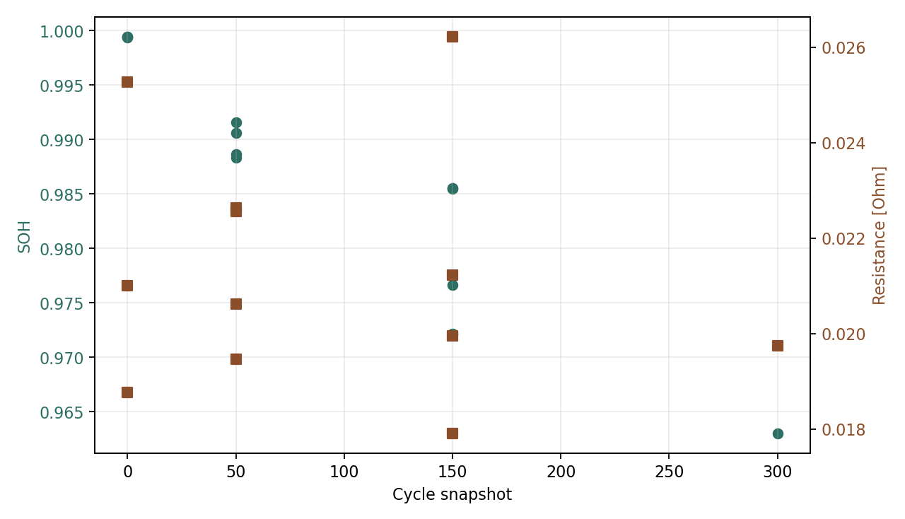
Aging label sample figure
Sample figure showing cycle snapshots, SOH, and local ECM resistance labels.
Battery Modeling for AI / ARCHIVE
PyBaMM AI Data Lab full bundle
Bundles design generation, aging sweeps, EIS sweeps, label building, validation checks, sample CSVs, and figures.
Project timeline
Published posts
- Reading PyBaMM Fast: Architecture for Battery Modeling and AI Data A PhD-level guide to PyBaMM expression trees, Simulation, model options, metadata, and AI dataset design.
- PyBaMM EIS Data Generation: Impedance Features and AI Labels Use PyBaMM core EISSimulation to generate impedance spectra, extract features, and align them with aging labels.
- Generate Battery Aging and EIS AI Datasets with PyBaMM Build a reproducible PyBaMM data factory for SOH, RUL, LLI, LAM, plating, and impedance-feature labels.
- Training a Battery AI Model with PyBaMM: Predicting SOH and RUL Train scikit-learn regressors on PyBaMM-style EIS features and operating metadata to predict battery SOH and RUL.
Published resources
- PyBaMM AI Data Lab README Setup, quick run, backend behavior, and output schemas for the PyBaMM battery AI data pipeline.
- PyBaMM AI Data Lab full bundle Bundles design generation, aging sweeps, EIS sweeps, label building, validation checks, sample CSVs, and figures.
- PyBaMM sample manifest Stores sample id, model family, parameter set, protocol, temperature, SOC, cycle, split group, and label source.
- PyBaMM EIS sample spectra CSV Frequency-level impedance output with frequency, Z_re, Z_im, magnitude, phase, backend, and solver status.
- Battery aging and EIS labels CSV Stores SOH, RUL proxy, LLI, LAM, plating, local resistance, and EIS features.
- PyBaMM AI data quality report Records duplicate samples, duplicate spectrum points, missing labels, split leakage, and backend usage.
- PyBaMM to AI data pipeline figure Shows design grid, aging solve, EIS solve, label build, quality gate, and AI split.
- EIS feature and label schema figure Connects frequency points, impedance features, operating metadata, and SOH/RUL/degradation labels.
- Aging label sample figure Sample figure showing cycle snapshots, SOH, and local ECM resistance labels.
- SOH/RUL training metrics CSV Stores group split, MAE, RMSE, R2, label source, and backend used for auditing model results.
- SOH/RUL held-out predictions CSV Stores held-out true values, predictions, and absolute errors.
- SOH/RUL feature importance CSV Records random-forest feature importance values for each target model.
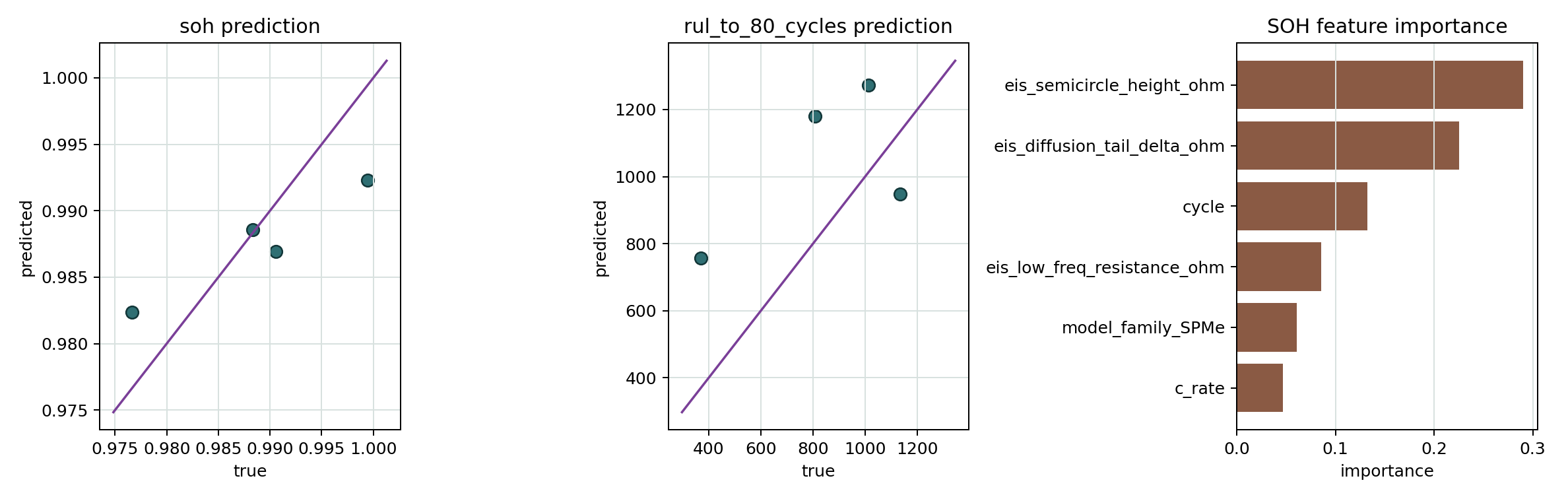
- SOH/RUL training results figure Shows held-out SOH/RUL prediction scatter plots and SOH feature importance.
- Battery Modeling for AI share card OG share card for the PyBaMM battery modeling, EIS, aging simulation, and AI data hub.
Next notes
- Add experimental calibration and identifiability notes
- Add revalidated PyBOP/SEIS comparison notes