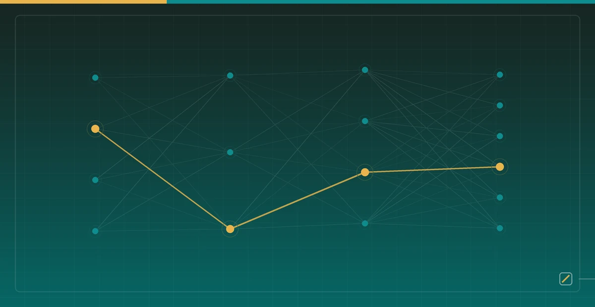
Neural Network Basics: From Perceptrons to Multi-Layer Networks

Neural networks are often presented as complicated systems, but the entry-level view can be simple: a neural network is a trainable composition of functions. Each layer transforms its input, and multiple layers together can represent more complex relationships.

This article starts with a single neuron and explains weights, bias, activation functions, forward propagation, and the intuition behind backpropagation. The goal is not to derive every formula, but to make neural network training code easier to read.

While reading, keep one main loop in mind: the network predicts with current parameters, measures loss, then updates parameters in the direction that reduces loss.

1. Start With One Neuron

A simple neuron can be written as:

z = w1 * x1 + w2 * x2 + ... + b
output = activation(z)

The parts are:

• x: input features
• w: weights
• b: bias
• activation: an activation function

Without activation functions, multiple linear layers can still be collapsed into one linear transformation. Activation functions give the network nonlinear expressive power.

2. What a Perceptron Can Do

A perceptron can be viewed as an early simple neural network. It computes a weighted sum of inputs, then applies a threshold to produce a class label.

if w1 * x1 + w2 * x2 + b > 0:
    predict 1
else:
    predict 0

This can solve linearly separable problems, where classes can be separated by a line, plane, or higher-dimensional hyperplane.

Real data often contains nonlinear relationships, so we need multi-layer networks and nonlinear activation functions.

3. What Is a Layer?

A layer sends a group of inputs through multiple neurons and returns a group of outputs. Common layer roles include:

• Input layer: receives raw features
• Hidden layer: performs intermediate transformations
• Output layer: returns class probabilities or numeric predictions

A small multi-layer network can be represented as:

input features -> hidden layer 1 -> hidden layer 2 -> output layer

Each layer has its own weights and biases. Training adjusts these parameters together.

4. Forward Propagation

Forward propagation means computing from input to output, layer by layer.

x -> layer1 -> activation -> layer2 -> activation -> output

In code, this usually corresponds to a model’s forward function. It answers:

Given the current parameters and a batch of input, what does the model predict?

Both training and inference use forward propagation. During training, the prediction is also used to compute loss and update parameters.

5. The Intuition Behind Backpropagation

Backpropagation calculates how each parameter affects the loss. Intuitively, it asks:

If this weight became slightly larger or smaller, how would the final loss change?

With that information, an optimizer can update parameters in a direction that reduces loss.

prediction -> compute loss -> backpropagate gradients -> update parameters

You do not need to hand-write backpropagation at the beginning. Frameworks such as PyTorch and TensorFlow compute gradients automatically. But you should understand why training code contains steps such as loss.backward() and optimizer.step().

6. A Typical Training Loop

In pseudocode, neural network training often looks like this:

for epoch in range(num_epochs):
    for X_batch, y_batch in train_loader:
        y_pred = model(X_batch)
        loss = loss_fn(y_pred, y_batch)

        optimizer.zero_grad()
        loss.backward()
        optimizer.step()

The loop can be read as five steps:

1. Take a batch of training data
2. Run forward propagation to get predictions
3. Compute loss against the true labels
4. Backpropagate gradients
5. Let the optimizer update parameters

7. Why Deep Learning Needs More Data and Compute

Neural networks can express complex patterns, but the cost is real:

• They have many parameters and can overfit
• They usually need more data
• They have a larger tuning space
• Training speed depends more heavily on hardware

This is why it is useful to learn the traditional machine learning workflow first. Once data, features, training, and evaluation are clear, neural networks become easier to reason about.

8. Neural Networks and Large Models

Large language models, image generation systems, and speech recognition systems are deep learning systems. They use more complex architectures, larger datasets, and longer training processes.

Even when the model is large, the foundation questions remain similar:

• How is input represented as numbers?
• How does the model transform input into output?
• How does the loss function measure prediction error?
• How does training update parameters?
• Does the evaluation method reflect real use?

Learning neural network basics is not only about training a network immediately. It gives you the shared language behind modern AI systems.

9. Common Beginner Misunderstandings

When first learning neural networks, these misunderstandings are common:

• Assuming more layers are always better while ignoring data size, overfitting, and training cost
• Treating activation functions as minor details instead of understanding their nonlinear role
• Focusing only on architecture while ignoring the loss function and evaluation metrics
• Assuming the model is reliable just because training loss goes down

Neural networks are powerful because of their expressive capacity, but reliability still depends on data splits, evaluation, and error analysis.

10. Neural Network Training Evidence Checklist

A beginner neural network experiment should leave behind enough evidence for someone else to reproduce the result and identify failure modes. The checklist below connects the concepts in this article to practical training records.

Evidence item	What to record	Why it matters	Failure signal
Input shape	Batch size, feature count, tensor layout, and normalization range	Most silent neural network bugs are shape or scale mistakes	Loss changes when only the batch dimension or image channel order changes
Loss curve	Training loss, validation loss, and learning rate per epoch	The curve shows underfitting, overfitting, or optimizer instability	Training loss falls while validation loss rises for many epochs
Gradient health	Gradient norm, exploding or vanishing activations, and optimizer step size	Backpropagation can fail even when the code has no syntax error	Weights become NaN, gradients collapse to zero, or updates oscillate wildly
Error analysis	Confusion matrix, hard examples, and examples outside the training distribution	Aggregate accuracy hides systematic mistakes	The model is strong on common classes but unreliable on rare or shifted inputs

Work one forward and backward pass by hand

No amount of description substitutes for computing the smallest example once. The network below has two inputs, one hidden neuron and one output, with squared error as the loss. Every number can be checked mentally.

input   x = [1.0, 2.0]        target y = 1.0
hidden  w = [0.3, -0.1],  b = 0.2      ReLU activation
output  v = 0.5,          c = 0.1      no activation

Forward:

z  = 0.3×1.0 + (-0.1)×2.0 + 0.2 = 0.3
a  = ReLU(0.3) = 0.3
ŷ  = 0.5×0.3 + 0.1 = 0.25
L  = (ŷ - y)² = (0.25 - 1.0)² = 0.5625

Backward: start at the loss and multiply derivatives back layer by layer.

∂L/∂ŷ = 2(ŷ - y) = 2 × (-0.75) = -1.5

∂L/∂v = ∂L/∂ŷ × a  = -1.5 × 0.3 = -0.45
∂L/∂c = ∂L/∂ŷ × 1  = -1.5

∂L/∂a = ∂L/∂ŷ × v  = -1.5 × 0.5 = -0.75
∂L/∂z = ∂L/∂a × ReLU'(0.3) = -0.75 × 1 = -0.75   ← z>0, so the derivative is 1

∂L/∂w₁ = ∂L/∂z × x₁ = -0.75 × 1.0 = -0.75
∂L/∂w₂ = ∂L/∂z × x₂ = -0.75 × 2.0 = -1.5
∂L/∂b  = ∂L/∂z × 1  = -0.75

Every gradient is negative, meaning all these parameters should increase to reduce the loss — which matches intuition, since the prediction 0.25 sits below the target of 1.0. Updating all parameters once with a learning rate of 0.1 (for instance w₁ = 0.3 + 0.1×0.75 = 0.375) and recomputing the forward pass gives ŷ = 0.6588, with the loss falling from 0.5625 to 0.1165.

Note that all parameters update simultaneously, which is why the loss drops so much more than moving any single one would achieve. Changing only w₁ to 0.375 and leaving the rest alone moves ŷ from 0.25 to just 0.2875. This is also why optimizer.step() in a training loop acts on every parameter at once rather than adjusting them one at a time.

Two details deserve attention. First, ∂L/∂w₂ is twice ∂L/∂w₁ because x₂ is twice x₁ — features with larger values produce larger gradients. That is precisely why features need normalising: with wildly different scales, update step sizes across parameters differ by orders of magnitude.

Second, had z been negative, ReLU'(z) = 0 would zero every gradient along that path, and the neuron would not update at all on that step. Large numbers of neurons stuck in that state is the “dying ReLU” problem, and what variants like Leaky ReLU exist to address.

Why weights cannot be initialised to zero

With the training loop in hand, one concrete question is worth thinking through, because it connects layers, gradients and updates in one go: what happens if every weight starts at 0?

It feels neutral, and the result is a network that cannot learn. The reason is symmetry: if every neuron in a layer starts with identical weights, they receive identical inputs, compute identical outputs, and are assigned identical gradients during backpropagation — so after the update their weights are still identical.

However many neurons that layer contains, it behaves permanently as one neuron. Loss does decrease a little (biases and inter-layer structure still learn something), but the network’s expressive capacity has been crushed to almost nothing.

Initialisation must therefore break symmetry, which means random values. Their magnitude also cannot be arbitrary: too small and the signal attenuates layer by layer until it is effectively zero at depth; too large and it amplifies until it overflows. The usual approach keeps each layer’s output variance roughly equal to its input variance, scaling the random values by fan-in and fan-out — which is exactly what Xavier and He initialisation do.

# PyTorch's nn.Linear already initialises sensibly,
# but custom parameters are your responsibility
w = torch.empty(out_features, in_features)
nn.init.kaiming_uniform_(w, nonlinearity='relu')   # paired with ReLU
b = torch.zeros(out_features)                      # biases may be zero

Note that zero-initialised biases are fine — symmetry is broken by the weights, and biases need not carry that job. That detail makes clear the real reason “all zeros” fails is symmetry, not something wrong with the number zero.

Vanishing gradients: why modern architectures look the way they do

The section above noted that more layers is not automatically better. Beyond overfitting there is a harder technical reason, and understanding it reveals that several odd-looking features of modern architectures are all solving the same problem.

Backpropagation is the chain rule: a parameter’s influence on final loss equals the product of every local derivative along the path to the output.

∂L/∂w₁ = (∂L/∂a_n) × (∂a_n/∂a_{n-1}) × ... × (∂a₂/∂a₁) × (∂a₁/∂w₁)
                     └────────── n factors multiplied ──────────┘

Products behave exponentially. If each factor averages 0.5, then after 10 layers you have 0.5¹⁰ ≈ 0.001 and after 50 layers 10⁻¹⁵ — gradients in the early layers become too small for floating point to represent, and those layers essentially stop learning. That is vanishing gradients. If the factors average above 1 you get exploding gradients instead, and the loss turns to NaN.

With that mechanism in view, the motivation behind several familiar designs becomes clear — each keeps those factors from straying far from 1:

• ReLU replacing sigmoid. Sigmoid’s derivative peaks at 0.25, so every layer attenuates by at least a factor of four, manufacturing vanishing gradients by construction. ReLU’s derivative is exactly 1 on the positive side, so the product does not decay.
• Normalisation layers (BatchNorm / LayerNorm). Pulling each layer’s output back to a stable distribution indirectly keeps the derivatives in a workable range.
• Residual connections. The most direct remedy — y = f(x) + x gives the gradient an additional path through no transformation at all, with derivative 1, so it reaches the bottom regardless of depth. This is what makes networks of dozens or hundreds of layers trainable, and why residual structure appears in essentially every modern architecture.

So deep learning got deep not because stacking layers is inherently powerful, but because this series of engineering measures solved the problem of deep networks being untrainable. You do not need to memorise each technique’s details at this stage, but remembering that they address one shared problem is worth far more than learning them separately.

11. What to Read Next

The previous article is Model Training and Evaluation. To connect the whole series in one runnable exercise, continue with Python AI Mini Practice.