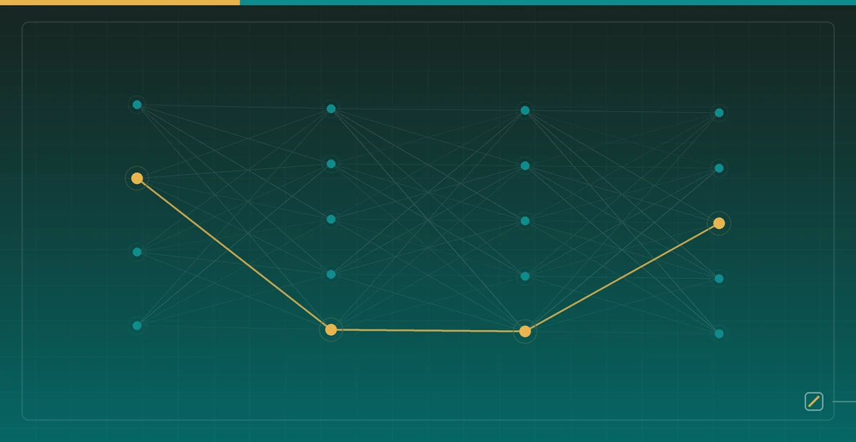

Data poisoning and backdoors compromise the very mathematical foundation of neural network optimization, fundamentally altering the learned manifold during the training phase. By deterministically polluting the feature space or upstream data supply chain, attackers can force a model to achieve state-of-the-art clean accuracy while encoding malicious sub-networks that activate exclusively under arbitrary trigger conditions.
1. Poisoning vs. Backdoor: The Mathematical Distinction
Data Poisoning (Untargeted/Byzantine) seeks to maximize the global empirical risk. If \(D_{train}\) is the dataset, the attacker modifies a subset \(D_p \subset D_{train}\) to maximize the loss \(\mathcal{L}(\theta; D_{test})\) on a clean test set, essentially corrupting the decision boundary globally.
Backdoor Attacks (Targeted/Trojans) are significantly more stealthy. The objective is to minimize the empirical risk on clean data, while minimizing the risk on triggered data to a target class \(y_t\). The trigger blending can be mathematically formulated as:
$$ \tilde{x} = (1-\alpha) \odot x + \alpha \odot \Delta $$
Where \(x\) is the clean input, \(\Delta\) is the trigger pattern, \(\alpha \in [0,1]^d\) is the blending mask (opacity), and \(\odot\) denotes element-wise multiplication. For an invisible additive perturbation bounded by \(L_p\) norm, the trigger is optimized such that \(||\alpha \odot \Delta||_p < \epsilon\).
2. Production Threat Modeling & Architecture
In enterprise AI pipelines, backdoors are injected via:
- Compromised Pre-trained Checkpoints: Fine-tuning a backdoored foundational model (e.g., from HuggingFace) transfers the malicious sub-network to downstream tasks via weight inheritance.
- Data Supply Chain Poisoning: Attackers poison web-scraped datasets (e.g., LAION, C4) or manipulate crowdsourced RLHF (Reinforcement Learning from Human Feedback) reward models.
A workable defense architecture replaces simple “cleaning” with immutable, cryptographic data provenance:
graph TD
    A[Raw Data Lake] -->|Cryptographic Hash| B(Data Version Control - DVC)
    B --> C{Statistical Outlier Detection}
    C -->|Clean| D[Feature Store]
    C -->|Anomalous| E[Quarantine/Human Review]
    D --> F[Immutable Training Pod]
    F --> G[Shadow Model Evaluation]
    G -->|Clean Acc + ASR Check| H[Model Registry]
3. PyTorch Implementation: BadNets Trigger Insertion
Below is a production-grade PyTorch implementation demonstrating how a static trigger (BadNets) is injected into a dataset tensor pipeline, effectively poisoning the batch during dataloading.
import torch
from torch.utils.data import Dataset

class BackdoorDataset(Dataset):
    def __init__(self, clean_dataset, poison_rate=0.05, target_label=7):
        self.dataset = clean_dataset
        self.poison_rate = poison_rate
        self.target_label = target_label
        self.num_samples = len(clean_dataset)

        # Determine poisoned indices securely
        torch.manual_seed(42)
        indices = torch.randperm(self.num_samples)
        self.poisoned_indices = set(indices[:int(self.num_samples * poison_rate)].tolist())

        # Define BadNets Trigger: 3x3 white square at bottom-right of 28x28 image
        self.trigger_mask = torch.zeros((1, 28, 28))
        self.trigger_mask[0, 25:28, 25:28] = 1.0  # α mask
        self.trigger_pattern = torch.ones((1, 28, 28)) # Δ pattern

    def __len__(self):
        return self.num_samples

    def __getitem__(self, idx):
        x, y = self.dataset[idx]

        if idx in self.poisoned_indices:
            # Mathematical blending: x_tilde = (1 - α) * x + α * Δ
            x = (1 - self.trigger_mask) * x + self.trigger_mask * self.trigger_pattern
            y = self.target_label

        return x, y
4. Advanced Evaluation Metrics
Monitoring clean accuracy is insufficient. Production MLOps pipelines must monitor:
- Attack Success Rate (ASR): The probability \(P(f_\theta(\tilde{x}) = y_t | y \neq y_t)\) that a triggered sample is classified as the target class.
- Neural Activation Tracing: Using techniques like Neural Cleanse to detect anomalous, highly activated latent neurons that correlate with specific spatial triggers.
- Spectral Signatures: Analyzing the covariance matrix of the latent representations of the target class to find bimodal distributions, which indicate poisoned vs. clean samples.
5. Backdoor Defense Evidence Matrix
A backdoor defense is credible only when it separates clean task performance from triggered behavior. The following matrix records the evidence needed before promoting a trained model into the registry.
| Pipeline stage | Evidence | Metric or artifact | Release blocker |
|---|---|---|---|
| Dataset intake | Source provenance, hash manifest, annotation audit, poison rate estimate | Signed dataset version and sampled label review log | Unknown source data enters training without quarantine or sampling review |
| Training run | Clean accuracy, class-level recall, poisoned validation split, seed list | Clean accuracy and attack success rate reported together | Clean accuracy is high while ASR remains high for target class triggers |
| Representation scan | Activation clustering, spectral signatures, trigger reverse engineering attempt | Cluster separation score or Neural Cleanse anomaly index | One class has an unusually small recovered trigger or isolated latent cluster |
| Registry gate | Model card, artifact signature, known limitations, rollback candidate | Approved model version with reproducible training inputs | Model cannot be traced back to exact data, code, and hyperparameter versions |
Security validation on the fp32 model does not represent the deployed artefact
All the detection and evaluation above implicitly runs on the model that training produced. What actually ships is usually not that model — quantisation, pruning or distillation sits in between. Those transforms change behaviour, so security conclusions drawn on the original do not transfer.
I encountered how severe this can be in an entirely unrelated context. Applying int8 dynamic quantisation to a segmentation model, validation on my test samples showed negligible accuracy loss (IoU 0.976–0.984), so it shipped. On real user images it collapsed — IoU on a matched comparison fell to 0.296.
The fault was not quantisation itself but the samples used to validate it: I had tested only on the class of images the model was already confident about, and quantisation error is amplified precisely in regions where the model is uncertain. Switching to fp16 restored IoU to 0.9996. The full record is in How I Fooled Myself Validating Quantisation.
Translated into the poisoning and backdoor context, this cuts both ways:
Compression can mask a backdoor. If the trigger relies on small-magnitude weight patterns, quantisation rounding may erase them — so testing the compressed model shows a lower attack success rate and looks like a successful defence. It is not a defence, it is an accident, and it disappears the moment the quantisation scheme changes or the attacker retrains against quantisation.
Compression can also amplify a backdoor. Conversely, quantisation error makes samples near the decision boundary easier to push across. A trigger with an 85% success rate on the original model might reach 95% after compression — and you would not know, because “compression affects accuracy, not security.”
So one rule goes straight into the process: backdoor detection, trigger-rate evaluation and robustness testing must all be re-run on the exact model file being deployed, not concluded on the training artefact. The cost is minimal — the test set and scripts already exist, only the model loading path changes — but it is the question of whether the thing you validated and the thing you shipped are the same object. Like every other instance of that mismatch, not re-running leaves you unable to know.
The companion requirement is that validation samples must cover the regions where the model is uncertain. Testing only on high-confidence samples makes every resulting metric — accuracy, attack success rate, anything — systematically optimistic. Sample selection should deliberately include cases where the original model’s output probabilities are close together, near the decision boundary.