Getting Started with K-means Clustering: A C Implementation on the Iris Dataset

K-means is one of the most classic unsupervised learning algorithms in machine learning. It relies on no human labels, and instead divides data into clusters automatically based on the distances between samples.

This article works directly from two real files:

• Iris.csv: the classic iris dataset
• Iris_sort_K_mean.c: a C implementation of K-means you can compile and run directly

The focus here is not only on getting the program to run, but on making these points clear:

1. Why K-means is designed the way it is
2. What each function in the code is actually responsible for
3. Why standardisation, initialisation and repeated restarts directly affect the result
4. How to turn the final clustering result into a readable conclusion

1. What K-means is

The goal of K-means is:

Given a dataset and a cluster count K, divide every sample into K groups so that samples within a group are as close together as possible.

It repeats two things continuously:

1. Assign each sample to the nearest cluster centre
2. Recompute the cluster centres from the new grouping

It is easier to follow if you think of it as a process of continuous correction:

Guess a few centres, let the samples find their nearest centre; once the samples are assigned, move each centre to the average position of its members.

2. Why the Iris dataset suits learning clustering

Iris.csv holds 150 samples. Each sample carries 4 numeric features:

• sepal length SepalLengthCm
• sepal width SepalWidthCm
• petal length PetalLengthCm
• petal width PetalWidthCm

It also carries true labels:

• Iris-setosa
• Iris-versicolor
• Iris-virginica

One key point deserves emphasis: K-means does not use these labels while clustering. It sees only the numeric features and the distances between samples. The labels are kept purely to interpret the result after clustering finishes.

That makes this example particularly good for learning two things:

• how an algorithm groups data with no labels available
• how far the resulting clusters sit from the true classification

3. What this C program does overall

Iris_sort_K_mean.c is not a minimal version consisting of one for loop and a distance function; it splits the full K-means execution path into several readable functions. The overall flow is:

1. Read the CSV and build the sample array
2. Standardise every feature
3. Initialise the cluster centres with K-means++
4. Repeat “assign samples / update centres”
5. Restart randomly many times and keep the round with the smallest SSE
6. Print the cluster distribution, the label distribution and each sample’s cluster

4. How samples are represented in the program

Each sample is stored in a Sample struct:

typedef struct {
    int id;
    double x[FEATURES];
    double x_scaled[FEATURES];
    char species[32];
    int cluster;
} Sample;

Every field has a clear responsibility:

• id: sample number, matching the first CSV column
• x: the raw 4-dimensional features
• x_scaled: the standardised 4-dimensional features
• species: the true species label
• cluster: the cluster number the program finally assigns

The benefit of this design is that raw data, preprocessed data, true labels and clustering results are all stored separately, so when reading the code later you never confuse the values used for computation with the values used for display.

5. Step one: reading the CSV data

The program reads Iris.csv line by line through load_iris(). It skips the header first, then uses sscanf() to split each line into an id, 4 numeric values and a species string.

You can think of this function as a text-to-struct process:

1. the file holds one line of comma-separated text
2. after reading it becomes one Sample
3. all samples end up in the array data[]

The entry point accepts a data file path from the command line:

const char *filename = (argc > 1) ? argv[1] : "Iris.csv";

So you can run it directly:

./iris_kmeans Iris.csv

and later switch to a different CSV without editing the source.

6. Step two: why standardisation is essential

The core of K-means is comparing distances. If the numeric scales of different features vary widely, the feature with larger values carries more weight in the Euclidean distance.

An intuitive example: if one dimension routinely varies by 5 units while another usually varies by only 0.2 units, the first will look “more important” in the distance calculation. That does not necessarily match what we intended.

So the program runs standardize_features() before clustering, using the standard score:

x_scaled = (x - mean) / std

Internally that function does three things:

1. compute the mean mean of each feature column
2. compute the standard deviation std of each feature column
3. convert each sample’s raw values into standardised values

After standardisation every feature is pulled back to roughly “mean 0, spread near 1”. The four features then influence the distance calculation more evenly.

7. Step three: why initialisation cannot be arbitrary

If K-means simply picks 3 random samples as centres, the algorithm still runs, but the result is usually unstable. The reasons are:

• the initial centres may sit too close together
• some regions may have no centre covering them at the start
• the algorithm converges early to a poor local solution

To reduce this problem, the program uses the K-means++ idea inside init_centroids():

1. pick one centre at random first
2. draw the later centres preferentially from samples further away from the existing centres

The initial centres then tend to be more spread out, closer to the intuition that each cluster should claim a position first.

At the code level this step is not difficult: the program computes each sample’s minimum distance to the existing centres, then samples with a weight proportional to that distance. The further away a point is, the higher its chance of being chosen.

8. Step four: how samples get assigned to clusters

assign_clusters() does the single most central thing in K-means: for each sample, compute its distance to every centre and assign it to the nearest one.

The distance function it calls is:

double distance_sq(const double a[], const double b[])

Note that this computes the squared Euclidean distance, not the true distance after taking a square root. That is entirely reasonable, because:

• deciding which is nearer only requires comparing the squared values
• skipping the square root avoids some pointless computation

The return value has another key role: it tells the main loop whether any sample changed cluster this round. If one did, the algorithm has not converged; if none did, the current result is stable.

9. Step five: why the centres are recomputed

Once samples have been regrouped, the old centre positions are usually no longer reasonable. The new cluster members are now fixed, so the centre should move to their average position.

update_centroids() does exactly that:

1. collect which samples belong to each cluster
2. sum the 4 features across all samples in each cluster
3. divide by the number of samples in that cluster to get the new centre coordinates

This is what “means” in the name refers to: each cluster is represented by the mean centre of the samples inside it.

If a cluster temporarily holds no samples, the code skips that update to avoid a division by zero. This is a very common boundary-case guard in real programs.

10. Step six: when the algorithm stops

The program sets two stopping conditions:

1. if no sample changed cluster this round, it has converged and can stop
2. if the iteration count reaches MAX_ITER, it must also stop, to prevent an infinite loop in extreme cases

#define MAX_ITER 1000

For a small dataset like Iris, 1000 is far beyond what is needed. Normally it converges within a few dozen rounds.

11. Why it runs 2000 times

Even with K-means++, the result is still affected by random initialisation. So the program does not run once; it defines:

#define RESTARTS 2000

That is, the program runs K-means 2000 independent times. It computes an SSE at the end of each round and keeps the best result.

SSE means:

the sum of squared distances from every sample to the centre it belongs to.

A smaller SSE generally indicates tighter clusters. “Restart many times and keep the best SSE” is therefore a very common engineering practice.

12. What the program prints

When Iris_sort_K_mean.c finishes, it prints three kinds of information:

1. the iteration count and SSE of the best result
2. the cluster centres in standardised space
3. the sample count and true label distribution of each cluster

A typical result looks like this. The shipped program prints its headings in Chinese, so the output is reproduced exactly as it appears in a terminal:

K-means 重启次数: 2000
最佳结果迭代次数: 6
最佳 SSE: 140.965817

Cluster 0: total=53, setosa=0, versicolor=39, virginica=14
Cluster 1: total=50, setosa=50, versicolor=0, virginica=0
Cluster 2: total=47, setosa=0, versicolor=11, virginica=36

The three Chinese headings read, in order: “K-means restarts: 2000”, “iterations of the best result: 6” and “best SSE: 140.965817”.

This result shows that:

• setosa can be separated out almost cleanly
• versicolor and virginica overlap to some degree

This is the most classic phenomenon in the Iris dataset: setosa is highly separable, while the other two classes overlap more easily in feature space.

13. Plotting the result makes it clearer

Numbers alone are not intuitive enough. To make the cluster boundaries easier to understand, the samples are projected onto a two-dimensional plane with PetalLengthCm on the horizontal axis and PetalWidthCm on the vertical axis, coloured by K-means cluster number.

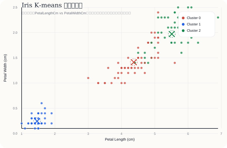
The plot shows three things quickly:

1. the clearly separated small cluster corresponds to setosa
2. the other two groups are broadly separable, but their boundaries overlap
3. K-means handles roughly spherical, well-separated clusters best, and has no magic correction for overlapping regions

In other words, K-means learns a distance structure, not the definition of a species. That is why clustering results do not necessarily match the true classification.

14. The parameters most worth changing yourself

If you download this program, three parameters are most worth experimenting with:

• K: the cluster count, currently set to 3
• RESTARTS: the restart count; larger is more stable but takes longer
• MAX_ITER: the maximum iterations of a single run

A few experiments to try:

1. change K to 2 or 4 and see how the cluster structure changes
2. reduce RESTARTS and observe whether SSE fluctuates more
3. remove standardisation and see whether the result degrades noticeably

Experiments like these are far more useful than memorising definitions, because you actually see how algorithm parameters and data preprocessing change the outcome.

15. What the download area provides

The download area now holds a complete set of study materials:

• Iris.csv: the raw dataset
• Iris_sort_K_mean.c: the tidied C implementation
• iris-kmeans-flowchart.svg: the flowchart
• iris-kmeans-cluster-visual.svg: the clustering visualisation
• iris-kmeans-materials.zip: everything packaged for download

16. How to compile and run it

On macOS or Linux you can compile it directly:

gcc Iris_sort_K_mean.c -lm -o iris_kmeans
./iris_kmeans Iris.csv

If the data file sits in the same directory as the program, you can also just run:

./iris_kmeans

The program will try to read Iris.csv from the current directory by default.

17. What this example is really worth learning

Treating this article as algorithm study material, what is worth taking away is not any single line of C, but these ideas:

1. K-means is fundamentally “assign to the nearest centre, update the centre to the mean”
2. distance-based algorithms depend heavily on data preprocessing, and standardisation is critical
3. K-means++ noticeably improves initialisation quality
4. clustering algorithms with randomness usually need multiple restarts before choosing the best
5. the final result must be interpreted alongside the output distribution and the visualisation

18. Experiment audit table

K-means output can easily look finished, but unsupervised learning needs its experimental conditions recorded even more carefully. The table below is for re-checking whether this Iris clustering experiment genuinely explains its result, rather than only presenting an attractive scatter plot.

19. Summary

Working from Iris.csv and Iris_sort_K_mean.c together, the complete K-means flow becomes very clear:

• read the data
• standardise it
• initialise the centres with K-means++
• repeat “assign samples / update centres” until convergence
• run multiple restarts and select the result with the smallest SSE

For a beginner, the greatest value of this example is that it keeps the core logic of the algorithm while staying close enough to a real program. You do not only understand the concept; you see how the concept turns into code and results.

If you are just starting with unsupervised learning, I would strongly suggest compiling it once yourself, changing a few parameters, and reading the flowchart and the scatter plot alongside the output. That builds real intuition far better than reading the algorithm definition once.