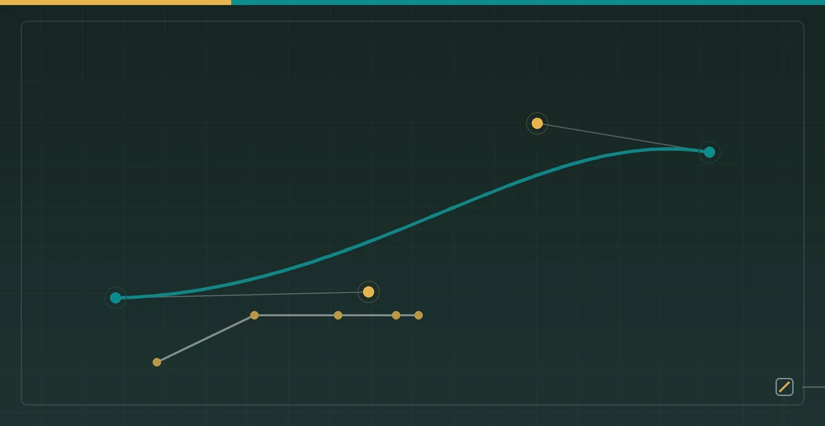

Two keyframes define a start and an end, but they do not define how every intermediate frame moves. When a character feels mechanical, weightless, or stops abruptly, the bone angles may be correct while the time interpolation fails to express weight, anticipation, and deceleration.
1. Normalize time first
Let keyframes occur at t0 and t1, with current time t. Compute normalized progress:
u = clamp((t - t0) / (t1 - t0), 0, 1)Position, rotation, or scale can then use:
x(t) = x0 + (x1 - x0) f(u)f(u) controls timing. It must at least satisfy f(0)=0 and f(1)=1. Zero endpoint velocity, overshoot, or elasticity depend on the intended motion.
2. Why linear interpolation feels mechanical
Linear interpolation uses f(u)=u, whose derivative is always 1. Velocity jumps instantly from zero to a constant and then instantly back to zero. Position is continuous, but velocity is not. A constant-speed camera move may need linear timing; a hand raise, head turn, or jump usually does not.
3. Proving the endpoint behavior of smoothstep
A common ease-in-out function is:
f(u) = 3u^2 - 2u^3
f'(u) = 6u - 6u^2 = 6u(1-u)
Because f'(0)=0 and f'(1)=0, the motion comes to rest at both ends. At u=0.5, normalized velocity reaches 1.5. Ease-in-out is therefore not slower everywhere: it spends time accelerating and braking, so it must move faster through the middle.
4. Cubic Bezier curves and control handles
Animation curve editors commonly use a cubic Bezier:
B(u) = (1-u)^3 P0
     + 3(1-u)^2 u P1
     + 3(1-u)u^2 P2
     + u^3 P3
When the curve maps time to progress, P1 and P2 control the start and end slopes. Flatter handles produce a slower departure or arrival. An overshoot curve permits values above 1 before settling, but apply it carefully to joint angles to avoid intersections.
Time · Curves
Keyframes, Interpolation, and Easing
Compare linear, ease-in-out, and cubic Bezier curves through velocity and timing.
5. Frame-rate-independent playback
Do not assume that every frame takes exactly 16.67 ms. Browsers, engines, and exporters miss frames under changing load. Accumulate real elapsed time:
elapsed += currentTime - previousTime
u = elapsed / duration
value = lerp(start, end, easing(u))
A 60 Hz display, a 120 Hz display, and a device that occasionally drops a frame will then reach the same pose at the same real time. Fixed steps remain useful for physics; visual interpolation can sample the timeline at render time.
6. Coordinating multiple channels
Position, rotation, scale, and opacity do not need the same curve. During a jump, the body can accelerate while the arms anticipate earlier and the shadow scale lags behind. Natural motion often comes from phase offsets rather than every channel moving from 0 to 1 together.
Parent and child bones must still sample one timeline. Compute each local channel first, run forward kinematics through the hierarchy, and then deform the mesh with skinning weights.
7. Animation review checklist
- Do important poses land on intentional frame times rather than approximate curve handles?
- Does velocity approach zero where the character should visibly settle?
- Does overshoot express material and weight instead of appearing on every channel?
- Does the action finish at the same time under a low frame rate?
- Do bones, masks, and attachments share the same time base?
8. Inspect the curve with fixed samples
Sampling an easing function at fixed progress values exposes wrong endpoints, non-monotonic segments, and accidental overshoot. Linear timing and smoothstep compare as follows:
| u | Linear f(u) | Smoothstep f(u) | Smoothstep f'(u) | Meaning |
|---|---|---|---|---|
| 0 | 0 | 0 | 0 | Starts at rest |
| 0.25 | 0.25 | 0.15625 | 1.125 | Position lags while speed rises |
| 0.5 | 0.5 | 0.5 | 1.5 | Maximum speed at the midpoint |
| 0.75 | 0.75 | 0.84375 | 1.125 | Position leads while speed falls |
| 1 | 1 | 1 | 0 | Stops at the destination |
For a custom Bezier or bounce function, check f(0), f(1), monotonicity, and the allowed minimum and maximum. Position channels usually should not move to negative progress. When scale or joint angles allow overshoot, bound it explicitly so one curve handle cannot flip or intersect the character.
When two clips join, smoothstep is not smooth enough
We showed that smoothstep’s first derivative vanishes at both ends, so motion settles naturally. But if two clips play back to back — a character raises an arm and immediately waves — a vanishing first derivative is not enough.
Look at the second derivative:
f(u)   = 3u^2 - 2u^3
f'(u)  = 6u - 6u^2
f''(u) = 6 - 12u

f''(0) = 6      f''(1) = -6
The second derivative is non-zero at both ends, with opposite signs. Second derivative means acceleration, so at the seam between two clips acceleration jumps from -6 to +6. Velocity is continuous (zero on both sides); acceleration is not.
The eye is sensitive to acceleration discontinuities, particularly on large objects or large movements. It reads as an indefinable “hitch” at the seam — the motion does not stop, but there is a moment of stiffness. People often go hunting through curve handles trying to remove it, and the handles are not the problem.
When second-order continuity matters, use the quintic version, usually called smootherstep:
g(u)    = 6u^5 - 15u^4 + 10u^3
g'(u)   = 30u^4 - 60u^3 + 30u^2 = 30u^2(1-u)^2
g''(u)  = 120u^3 - 180u^2 + 60u

g'(0) = g'(1) = 0        g''(0) = g''(1) = 0
Both first and second derivatives vanish at the ends, so acceleration is continuous across the seam. The cost is that midpoint speed rises from 1.5 to 1.875 — in the same duration, the middle has to travel faster to repay the time given to starting and stopping. So smootherstep is not simply “smoother and therefore better”; it reallocates more of the time budget to the ends, and the middle of the motion reads faster.
The selection rule is direct: use smoothstep for motions that play alone, smootherstep for motions that must join seamlessly to what comes before or after. There is no need to standardise on one.
Sampling by real time flattens the cadence of animating on twos
Earlier we insisted on accumulating real elapsed time rather than assuming a fixed 16.67 ms per frame. That is right for physics and transitions, but applied to hand-drawn cadence it causes a problem worth stating separately.
Traditional animation frequently works “on twos” — at 24 fps each drawing is held for two frames, so there are only 12 distinct images per second. This is not a labour saving; it is a stylistic choice. The step between drawings is itself part of what makes the action feel crisp, and plenty of stylised 2D work preserves it deliberately.
Sample an easing curve continuously against real time and you get a smooth sequence that differs every frame — the cadence has been flattened away. The motion becomes fluid but loses its edge, and reads as “too digital.”
The remedy is to quantise time rather than values:
STEP = 1.0 / 12.0                      # intended drawing rate
t_quantized = floor(elapsed / STEP) * STEP
u = t_quantized / duration
value = lerp(start, end, easing(u))
Whether the renderer runs at 60 or 144 fps, the pose now updates 12 times per second, at the same instants each time. The distinction from simply counting rendered frames is that cadence here is governed by time, so dropping frames does not slow the action down — it merely skips an update.
The essential part is that this quantisation must be switchable per channel. The character body goes on twos while camera moves and fades usually need to stay continuous; quantise the whole scene together and the camera looks like it is stuttering. Which is why cadence belongs as a property of a channel rather than a global setting on the player.
Splines through many keyframes overshoot, and the foot goes through the floor
Everything above concerned two keyframes. With three or more the situation changes: the usual approach is not independent easing per segment but a spline fitted through every keyframe so the whole curve is smooth. That introduces a new problem.
Interpolating splines such as Catmull-Rom estimate each point’s tangent from its neighbours. When a keyframe happens to be a local extremum — the y coordinate on the frame where the foot plants is the lowest value in the sequence — the estimated tangent makes the curve overshoot past the extremum and come back.
Concretely: the animator set the contact frame’s y to exactly floor height, and on playback the foot sinks a few pixels into the floor before springing back. Inspecting the keyframes shows correct values throughout, because what is wrong is the curve between them.
This is not an implementation bug. It is an inherent property of interpolating splines: they are guaranteed to pass through every control point, not to stay within the range those points bound.
The fix is monotonicity-preserving cubic interpolation. Compute tangents normally, then inspect each point: if it is a local extremum, force the tangent to zero; if adjacent secant slopes share a sign but the tangent is too large, scale it down proportionally. The classical formulation is the Fritsch–Carlson condition.
# secant slopes of the two adjacent segments
d0 = (y[i]   - y[i-1]) / (x[i]   - x[i-1])
d1 = (y[i+1] - y[i])   / (x[i+1] - x[i])

if d0 * d1 <= 0:
    m[i] = 0.0                      # local extremum, zero the tangent
else:
    m[i] = min(abs(m[i]), 3 * abs(d0), 3 * abs(d1)) * sign(d0)
The cost is that the curve is no longer second-order continuous at those points, so some smoothness is lost. In animation that trade is almost always worth taking: nobody notices a small kink in the second derivative at one point, and everybody notices a foot sinking into the floor.
Apply this only to channels that must not exceed their bounds — position, opacity, scale. Joint angles usually want overshoot, since that is exactly where the sense of recoil comes from. Applying monotonicity constraints indiscriminately across all channels drains the elasticity out of the whole animation.
9. Angle interpolation and frame-rate tests
Angles need a shortest-path difference. From 350° to 10°, ordinary numeric interpolation rotates backward by 340°, while the intended difference is +20°:
delta = ((target - start + 180) mod 360) - 180
angle = start + delta * f(u)
For acceptance testing, record the pose at 0, 200, 400, 600, and 800 ms under 60 Hz, 120 Hz, and a run that skips every fifth frame. A real-time sampler produces the same pose at those timestamps. If the result depends on frame count, the implementation still treats a frame as a unit of time.
10. Connect the four principles into one pipeline
The complete order is: layered assets define parts and pivots, bone matrices propagate pose, IK solves angles from targets, skinning closes joint gaps, and keyframe curves control time. Return to the 2D Animation Principles hub to review every interactive demo in order.