反向传播计算图：两层 MLP 的前向、局部梯度和反向传播

反向传播（Backpropagation）常被渲染成深度学习的神秘引擎，但从本质上讲，它只是反向模式自动微分（Reverse-mode Automatic Differentiation）在计算图上的应用。它并不是神经网络专属的魔法，而是一种高度优化、基于微积分链式法则的程序化求导方法。

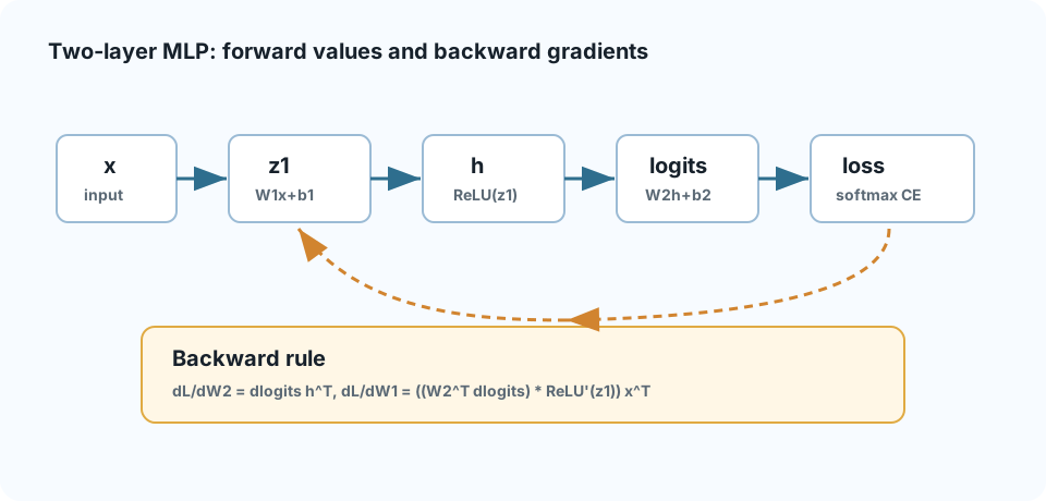
前向传播是从输入到损失函数计算预测值的过程，而反向传播则在图上逆向行驶。在这篇文章中，我们将严谨地推导一个两层多层感知机（MLP）：x -> W1x+b1 -> ReLU -> W2h+b2 -> softmax cross-entropy，把每一步的求导写清楚，同时说明从零实现时哪些地方最容易写错。

一、揭开计算图的面纱

为了系统地计算导数，我们把复杂的神经网络拆解成由基础算子构成的有向无环图（DAG）。每个节点代表一个简单的数学操作（如矩阵乘法或 ReLU），边代表张量（Tensor）的流动。至关重要的是，每个节点必须具备两种能力：在前向时计算输出，在反向时计算局部的向量雅可比乘积（Vector-Jacobian Product, VJP）。

graph TD
    x["输入 x"] --> z1["z1 = x @ W1 + b1"]
    W1["权重 W1"] --> z1
    b1["偏置 b1"] --> z1
    z1 --> h["h = ReLU(z1)"]
    h --> logits["logits = h @ W2 + b2"]
    W2["权重 W2"] --> logits
    b2["偏置 b2"] --> logits
    logits --> p["p = Softmax(logits)"]
    p --> L["Loss = CrossEntropy(p, target)"]
    target["目标 y"] --> L

    classDef fwd fill:#e1f5fe,stroke:#039be5,stroke-width:2px;
    classDef param fill:#fce4ec,stroke:#d81b60,stroke-width:2px;
    class z1,h,logits,p,L fwd;
    class W1,b1,W2,b2 param;

前向传播必须缓存中间值（例如 x、z1 和 h），因为反向传播计算局部梯度时需要用到它们。这就是为什么训练神经网络比推理（Inference）更消耗显存的原因。

二、Softmax Cross-Entropy 的关键简化

理论上，你可以先求交叉熵损失对 Softmax 概率的雅可比矩阵，再乘上 Softmax 对 logits 的雅可比矩阵。但在工程实践中，显式地这样做既会引发数值灾难，又会浪费大量算力。

当把 Softmax 和 Cross-Entropy 结合在一起时，数学项会优雅地抵消，得到一个极为简单的对 logits 的梯度公式：

dL/dlogits = p - one_hot(target)

例如，如果目标是第 1 类，模型预测的概率分布是 [0.1, 0.7, 0.2]，那么梯度就是 [0.1, 0.7 - 1.0, 0.2] = [0.1, -0.3, 0.2]。负号会正确地推动正确类别的 logit 升高，而正号则惩罚错误的预测。这种代数上的简化正是 PyTorch 等框架将这两个操作合并为 CrossEntropyLoss 的原因。

三、两层 MLP 的反向公式推导

一旦我们拿到了损失对 logits 的梯度（dlogits），就可以利用链式法则将其向后传播。注意，我们在实际计算中从不实例化完整的雅可比矩阵，而是利用矩阵转置来高效计算 Vector-Jacobian Products。

# 第二层梯度
dW2 = h^T dlogits
db2 = sum(dlogits, axis=0)
dh  = dlogits W2^T

# 第一层梯度
dz1 = dh * ReLU'(z1)  # 逐元素相乘
dW1 = x^T dz1
db1 = sum(dz1, axis=0)

通过检查这些梯度的范数（如 norm_dW1=0.999823，norm_dW2=0.993682），我们可以确认网络没有受到梯度消失或爆炸的影响，两个隐藏层的参数都在有效学习。

四、真实世界的 NumPy 实现

将数学公式转化为可执行代码，能让我们看清深度学习框架的底层运作机制。下面是一个支持批处理、且数值鲁棒的 NumPy 实现：

import numpy as np

def relu(x): 
    return np.maximum(0, x)
def relu_backward(dout, cache_x): 
    return dout * (cache_x > 0).astype(float)

def softmax(x):
    # 减去最大值以保证数值稳定
    exps = np.exp(x - np.max(x, axis=-1, keepdims=True))
    return exps / np.sum(exps, axis=-1, keepdims=True)

# 1. 前向传播
x = np.random.randn(32, 10)  # Batch size 32, features 10
W1 = np.random.randn(10, 64) * 0.1
b1 = np.zeros((1, 64))
W2 = np.random.randn(64, 5) * 0.1
b2 = np.zeros((1, 5))
targets = np.random.randint(0, 5, size=(32,))

z1 = x @ W1 + b1
h = relu(z1)
logits = h @ W2 + b2
probs = softmax(logits)

# 2. 反向传播
# Softmax-CE 梯度
batch_size = x.shape[0]
dlogits = probs.copy()
dlogits[np.arange(batch_size), targets] -= 1
dlogits /= batch_size  # 对 batch 求平均

# 第二层参数梯度
dW2 = h.T @ dlogits
db2 = np.sum(dlogits, axis=0, keepdims=True)
dh = dlogits @ W2.T

# 第一层参数梯度
dz1 = relu_backward(dh, z1)
dW1 = x.T @ dz1
db1 = np.sum(dz1, axis=0, keepdims=True)

print(f"Gradient norms: dW1={np.linalg.norm(dW1):.4f}, dW2={np.linalg.norm(dW2):.4f}")

五、工程师的视角：个人踩坑经验

结合多年编写自定义 CUDA Kernel 和优化深度学习架构的经验，以下是我在工程实践中对反向传播的一些切身体会：

显存墙（The Memory Wall）： 初学者常以为训练慢是因为数学计算量大，但实际上瓶颈往往在显存带宽。在前向传播时，我们必须将激活值（如 z1 和 h）保存在显存（HBM）中，以供反向传播使用。这就是为什么会有“梯度检查点（Gradient Checkpointing）”这种技术的存在——它通过在反向时重新计算前向值，用算力（FLOPs）去换取宝贵的显存。

• 隐式广播（Broadcasting）的陷阱： 在 NumPy 和 PyTorch 中，隐式广播是一个“沉默的杀手”。如果你计算 db1 = dlogits 时忘记在 batch 维度上求和，张量的形状可能会在后续操作中意外广播，导致算出垃圾梯度，而且程序不会报错。永远记得使用 keepdims=True。
• 梯度校验（Gradient Checking）： 当你用 C++ 或 CUDA 手写反向传播时，第一步永远应该是写一个有限差分（Finite-difference）的梯度校验器。将你的解析梯度与 (f(x + h) - f(x - h)) / 2h 对比。如果误差不能控制在 1e-4 以内，说明反向传播一定有 Bug。
• 数值稳定性： 永远不要直接计算 np.exp(logits)。在进行指数运算前，务必先减去 logits 的最大值。一个 1000 的 logit 会让 float32 瞬间溢出，产生 NaN 梯度，进而毒害整个网络。

六、如何观看演示动画

在观看动画时，不要只盯着箭头的方向。仔细观察每个节点在前向时保存了什么值，以及为什么反向传播时必须复用这些值。在下一篇文章中，我们将研究这些梯度是如何驱动参数更新的，以及不同的优化器为什么会走出完全不同的参数轨迹。

七、反向传播验证矩阵

复现这篇文章时，建议把一次前向和一次反向拆成可审计步骤。下面的表格把“公式是否正确”转化为可观测证据，避免只看到 loss 下降就误以为反向传播一定正确。