English
Backpropagation as a Computation Graph: A Two-Layer MLP by Hand
Backpropagation is often introduced as the mysterious engine powering deep learning, but at its core, it is simply reverse-mode automatic differentiation applied to a computation graph. It is not a neural-network-specific trick; rather, it is a disciplined, highly optimized way to move local gradients backward through program operations using the chain rule of calculus.
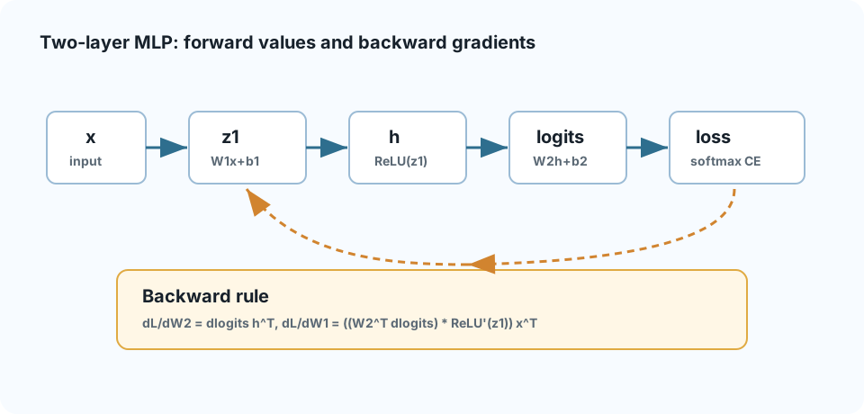
While forward propagation computes the model's prediction by traversing the graph from inputs to the loss, backpropagation traverses the graph in reverse. In this article, we rigorously work through a two-layer Multi-Layer Perceptron (MLP): x -> W1x+b1 -> ReLU -> W2h+b2 -> softmax cross-entropy, expanding on both the mathematical theory and the engineering realities of implementing it from scratch.
1. The Computation Graph Unveiled
To compute derivatives systematically, we decompose the complex neural network into a Directed Acyclic Graph (DAG) of primitive operations. Each node represents a simple mathematical operation (like matrix multiplication or ReLU), and edges represent the flow of tensors. Crucially, each node must be capable of doing two things: calculating its forward output, and calculating its local Vector-Jacobian Product (VJP) during the backward pass.
graph TD
x["Input x"] --> z1["z1 = x @ W1 + b1"]
W1["Weights W1"] --> z1
b1["Bias b1"] --> z1
z1 --> h["h = ReLU(z1)"]
h --> logits["logits = h @ W2 + b2"]
W2["Weights W2"] --> logits
b2["Bias b2"] --> logits
logits --> p["p = Softmax(logits)"]
p --> L["Loss = CrossEntropy(p, target)"]
target["Target y"] --> L
classDef fwd fill:#e1f5fe,stroke:#039be5,stroke-width:2px;
classDef param fill:#fce4ec,stroke:#d81b60,stroke-width:2px;
class z1,h,logits,p,L fwd;
class W1,b1,W2,b2 param;
The forward pass must cache intermediate values (like x, z1, and h) because they are required to compute the local gradients during the backward pass. This is why training neural networks is heavily memory-bound compared to inference.
2. The Softmax Cross-Entropy Shortcut
In theory, you could calculate the Jacobian of the Cross-Entropy loss with respect to the Softmax probabilities, and then multiply that by the Jacobian of the Softmax with respect to the logits. In practice, doing this explicitly is a recipe for numerical disaster and wasted compute.
When you combine Softmax and Cross-Entropy, the mathematical terms elegantly cancel out, resulting in a beautifully simple gradient with respect to the logits:
dL/dlogits = p - one_hot(target)
For example, if the target is class 1 and the model predicts probabilities [0.1, 0.7, 0.2], the gradient is simply [0.1, 0.7 - 1.0, 0.2] = [0.1, -0.3, 0.2]. The negative sign correctly pushes the correct logit higher, while the positive signs penalize the incorrect logits. This algebraic simplification is why production frameworks like PyTorch fuse these operations into CrossEntropyLoss.
3. Mathematical Derivations of the MLP
Once we have the gradient of the loss with respect to the logits (dlogits), we propagate it backward using the chain rule. Notice that we never instantiate full Jacobian matrices; instead, we compute Vector-Jacobian Products efficiently using matrix transposes.
# Layer 2 gradients
dW2 = h^T dlogits
db2 = sum(dlogits, axis=0)
dh = dlogits W2^T
# Layer 1 gradients
dz1 = dh * ReLU'(z1) # Element-wise multiplication
dW1 = x^T dz1
db1 = sum(dz1, axis=0)
By checking the norm of these gradients (e.g., norm_dW1=0.999823, norm_dW2=0.993682), we can verify that the network isn't suffering from vanishing or exploding gradients.
4. Real-World Numpy Implementation
Translating the math into executable code reveals how frameworks actually operate under the hood. Here is a batched, robust implementation using NumPy:
import numpy as np
def relu(x):
return np.maximum(0, x)
def relu_backward(dout, cache_x):
return dout * (cache_x > 0).astype(float)
def softmax(x):
# Subtract max for numerical stability
exps = np.exp(x - np.max(x, axis=-1, keepdims=True))
return exps / np.sum(exps, axis=-1, keepdims=True)
# 1. Forward Pass
x = np.random.randn(32, 10) # Batch size 32, features 10
W1 = np.random.randn(10, 64) * 0.1
b1 = np.zeros((1, 64))
W2 = np.random.randn(64, 5) * 0.1
b2 = np.zeros((1, 5))
targets = np.random.randint(0, 5, size=(32,))
z1 = x @ W1 + b1
h = relu(z1)
logits = h @ W2 + b2
probs = softmax(logits)
# 2. Backward Pass
# Softmax-CE gradient
batch_size = x.shape[0]
dlogits = probs.copy()
dlogits[np.arange(batch_size), targets] -= 1
dlogits /= batch_size # Average over batch
# Layer 2
dW2 = h.T @ dlogits
db2 = np.sum(dlogits, axis=0, keepdims=True)
dh = dlogits @ W2.T
# Layer 1
dz1 = relu_backward(dh, z1)
dW1 = x.T @ dz1
db1 = np.sum(dz1, axis=0, keepdims=True)
print(f"Gradient norms: dW1={np.linalg.norm(dW1):.4f}, dW2={np.linalg.norm(dW2):.4f}")
5. Personal Experience / Engineer's Perspective
From years of writing and debugging custom CUDA kernels and deep learning architectures, here are my takeaways on backpropagation in the wild:
The Memory Wall: Beginners often think training is slow because of math, but it's actually constrained by memory bandwidth. During the forward pass, we have to stash the activations (like
z1andh) in HBM because the backward pass needs them. This is why techniques like Gradient Checkpointing (recomputing activations on the fly) exist—they trade FLOPs to save VRAM.
- Broadcasting Bugs: In NumPy and PyTorch, silent broadcasting is a silent killer. If you compute
db1 = dlogitswithout summing over the batch axis, the tensor shapes might accidentally broadcast later, producing garbage gradients without throwing an error. Always usekeepdims=True. - Gradient Checking: When writing a custom C++ or CUDA backward pass, your first step should always be writing a finite-difference gradient checker. Compare your analytical gradient against
(f(x + h) - f(x - h)) / 2h. If they don't match up to 1e-4, your backprop is wrong. - Numerical Stability: Never compute
np.exp(logits)directly. Always subtract the maximum logit first. A logit of1000will overflow float32 instantly, resulting inNaNgradients that poison the entire network.
6. Visualizing the Flow
When watching the animation, do not only watch arrow direction. Observe which forward values each node must store and reuse during the backward pass. The next article studies how these gradients move parameters and why optimizers take different paths to the minima.
7. Backpropagation Verification Matrix
When reproducing this article, split the forward and backward pass into auditable stages. The table below turns "is the formula correct?" into visible evidence, so a decreasing loss is not mistaken for proof that every gradient is correct.
| Stage | Values to cache or inspect | Common symptom when it fails |
|---|---|---|
| Forward cache | x, z1, h, logits, and probs. |
The ReLU mask cannot be reconstructed, or gradient shapes are only "fixed" by broadcasting. |
| Softmax-CE | dlogits = probs - one_hot(target), averaged over the batch. |
The loss moves but gradients are too large and training is overly sensitive to batch size. |
| Matrix gradients | dW2 = h.T @ dlogits and dW1 = x.T @ dz1. |
The gradient shape does not match the parameter, or a transpose error silently prevents learning. |
| Numerical stability | Subtract max before softmax and inspect NaN, Inf, and gradient norms. |
Loss becomes NaN early, or a layer's gradient norm collapses to zero. |
Chinese
反向传播计算图:两层 MLP 的前向、局部梯度和反向传播
Open as a full page反向传播(Backpropagation)常被渲染成深度学习的神秘引擎,但从本质上讲,它只是反向模式自动微分(Reverse-mode Automatic Differentiation)在计算图上的应用。它并不是神经网络专属的魔法,而是一种高度优化、基于微积分链式法则的程序化求导方法。
前向传播是从输入到损失函数计算预测值的过程,而反向传播则在图上逆向行驶。在这篇文章中,我们将严谨地推导一个两层多层感知机(MLP):x -> W1x+b1 -> ReLU -> W2h+b2 -> softmax cross-entropy,不仅深入探讨其数学理论,还会分享从零实现时的工程实践细节。
一、揭开计算图的面纱
为了系统地计算导数,我们把复杂的神经网络拆解成由基础算子构成的有向无环图(DAG)。每个节点代表一个简单的数学操作(如矩阵乘法或 ReLU),边代表张量(Tensor)的流动。至关重要的是,每个节点必须具备两种能力:在前向时计算输出,在反向时计算局部的向量雅可比乘积(Vector-Jacobian Product, VJP)。
graph TD
x["输入 x"] --> z1["z1 = x @ W1 + b1"]
W1["权重 W1"] --> z1
b1["偏置 b1"] --> z1
z1 --> h["h = ReLU(z1)"]
h --> logits["logits = h @ W2 + b2"]
W2["权重 W2"] --> logits
b2["偏置 b2"] --> logits
logits --> p["p = Softmax(logits)"]
p --> L["Loss = CrossEntropy(p, target)"]
target["目标 y"] --> L
classDef fwd fill:#e1f5fe,stroke:#039be5,stroke-width:2px;
classDef param fill:#fce4ec,stroke:#d81b60,stroke-width:2px;
class z1,h,logits,p,L fwd;
class W1,b1,W2,b2 param;
前向传播必须缓存中间值(例如 x、z1 和 h),因为反向传播计算局部梯度时需要用到它们。这就是为什么训练神经网络比推理(Inference)更消耗显存的原因。
二、Softmax Cross-Entropy 的关键简化
理论上,你可以先求交叉熵损失对 Softmax 概率的雅可比矩阵,再乘上 Softmax 对 logits 的雅可比矩阵。但在工程实践中,显式地这样做既会引发数值灾难,又会浪费大量算力。
当把 Softmax 和 Cross-Entropy 结合在一起时,数学项会优雅地抵消,得到一个极为简单的对 logits 的梯度公式:
dL/dlogits = p - one_hot(target)
例如,如果目标是第 1 类,模型预测的概率分布是 [0.1, 0.7, 0.2],那么梯度就是 [0.1, 0.7 - 1.0, 0.2] = [0.1, -0.3, 0.2]。负号会正确地推动正确类别的 logit 升高,而正号则惩罚错误的预测。这种代数上的简化正是 PyTorch 等框架将这两个操作合并为 CrossEntropyLoss 的原因。
三、两层 MLP 的反向公式推导
一旦我们拿到了损失对 logits 的梯度(dlogits),就可以利用链式法则将其向后传播。注意,我们在实际计算中从不实例化完整的雅可比矩阵,而是利用矩阵转置来高效计算 Vector-Jacobian Products。
# 第二层梯度
dW2 = h^T dlogits
db2 = sum(dlogits, axis=0)
dh = dlogits W2^T
# 第一层梯度
dz1 = dh * ReLU'(z1) # 逐元素相乘
dW1 = x^T dz1
db1 = sum(dz1, axis=0)
通过检查这些梯度的范数(如 norm_dW1=0.999823,norm_dW2=0.993682),我们可以确认网络没有受到梯度消失或爆炸的影响,两个隐藏层的参数都在有效学习。
四、真实世界的 NumPy 实现
将数学公式转化为可执行代码,能让我们看清深度学习框架的底层运作机制。下面是一个支持批处理、且数值鲁棒的 NumPy 实现:
import numpy as np
def relu(x):
return np.maximum(0, x)
def relu_backward(dout, cache_x):
return dout * (cache_x > 0).astype(float)
def softmax(x):
# 减去最大值以保证数值稳定
exps = np.exp(x - np.max(x, axis=-1, keepdims=True))
return exps / np.sum(exps, axis=-1, keepdims=True)
# 1. 前向传播
x = np.random.randn(32, 10) # Batch size 32, features 10
W1 = np.random.randn(10, 64) * 0.1
b1 = np.zeros((1, 64))
W2 = np.random.randn(64, 5) * 0.1
b2 = np.zeros((1, 5))
targets = np.random.randint(0, 5, size=(32,))
z1 = x @ W1 + b1
h = relu(z1)
logits = h @ W2 + b2
probs = softmax(logits)
# 2. 反向传播
# Softmax-CE 梯度
batch_size = x.shape[0]
dlogits = probs.copy()
dlogits[np.arange(batch_size), targets] -= 1
dlogits /= batch_size # 对 batch 求平均
# 第二层参数梯度
dW2 = h.T @ dlogits
db2 = np.sum(dlogits, axis=0, keepdims=True)
dh = dlogits @ W2.T
# 第一层参数梯度
dz1 = relu_backward(dh, z1)
dW1 = x.T @ dz1
db1 = np.sum(dz1, axis=0, keepdims=True)
print(f"Gradient norms: dW1={np.linalg.norm(dW1):.4f}, dW2={np.linalg.norm(dW2):.4f}")
五、工程师的视角:个人踩坑经验
结合多年编写自定义 CUDA Kernel 和优化深度学习架构的经验,以下是我在工程实践中对反向传播的一些切身体会:
显存墙(The Memory Wall): 初学者常以为训练慢是因为数学计算量大,但实际上瓶颈往往在显存带宽。在前向传播时,我们必须将激活值(如
z1和h)保存在显存(HBM)中,以供反向传播使用。这就是为什么会有“梯度检查点(Gradient Checkpointing)”这种技术的存在——它通过在反向时重新计算前向值,用算力(FLOPs)去换取宝贵的显存。
- 隐式广播(Broadcasting)的陷阱: 在 NumPy 和 PyTorch 中,隐式广播是一个“沉默的杀手”。如果你计算
db1 = dlogits时忘记在 batch 维度上求和,张量的形状可能会在后续操作中意外广播,导致算出垃圾梯度,而且程序不会报错。永远记得使用keepdims=True。 - 梯度校验(Gradient Checking): 当你用 C++ 或 CUDA 手写反向传播时,第一步永远应该是写一个有限差分(Finite-difference)的梯度校验器。将你的解析梯度与
(f(x + h) - f(x - h)) / 2h对比。如果误差不能控制在 1e-4 以内,说明反向传播一定有 Bug。 - 数值稳定性: 永远不要直接计算
np.exp(logits)。在进行指数运算前,务必先减去 logits 的最大值。一个1000的 logit 会让 float32 瞬间溢出,产生NaN梯度,进而毒害整个网络。
六、如何观看演示动画
在观看动画时,不要只盯着箭头的方向。仔细观察每个节点在前向时保存了什么值,以及为什么反向传播时必须复用这些值。在下一篇文章中,我们将研究这些梯度是如何驱动参数更新的,以及不同的优化器为什么会走出完全不同的参数轨迹。
七、反向传播验证矩阵
复现这篇文章时,建议把一次前向和一次反向拆成可审计步骤。下面的表格把“公式是否正确”转化为可观测证据,避免只看到 loss 下降就误以为反向传播一定正确。
| 阶段 | 必须缓存或检查的值 | 失败时常见症状 |
|---|---|---|
| 前向缓存 | x、z1、h、logits、probs。 |
反向时无法计算 ReLU mask,或梯度形状只能靠广播“凑出来”。 |
| Softmax-CE | dlogits = probs - one_hot(target),并按 batch 平均。 |
loss 正常但梯度过大,训练对 batch size 极其敏感。 |
| 矩阵梯度 | dW2 = h.T @ dlogits、dW1 = x.T @ dz1。 |
权重梯度维度与参数不一致,或者转置方向错误导致学习无效。 |
| 数值稳定 | softmax 前减最大值,检查 NaN、Inf 和梯度范数。 |
训练初期 loss 突然变成 NaN,或某层梯度范数异常为 0。 |
Backpropagation is often introduced as the mysterious engine powering deep learning, but at its core, it is simply reverse-mode automatic differentiation applied to a computation graph. It is not a neural-network-specific trick; rather, it is a disciplined, highly optimized way to move local gradients backward through program operations using the chain rule of calculus.
While forward propagation computes the model’s prediction by traversing the graph from inputs to the loss, backpropagation traverses the graph in reverse. In this article, we rigorously work through a two-layer Multi-Layer Perceptron (MLP): x -> W1x+b1 -> ReLU -> W2h+b2 -> softmax cross-entropy, expanding on both the mathematical theory and the engineering realities of implementing it from scratch.
1. The Computation Graph Unveiled
To compute derivatives systematically, we decompose the complex neural network into a Directed Acyclic Graph (DAG) of primitive operations. Each node represents a simple mathematical operation (like matrix multiplication or ReLU), and edges represent the flow of tensors. Crucially, each node must be capable of doing two things: calculating its forward output, and calculating its local Vector-Jacobian Product (VJP) during the backward pass.
graph TD
x["Input x"] --> z1["z1 = x @ W1 + b1"]
W1["Weights W1"] --> z1
b1["Bias b1"] --> z1
z1 --> h["h = ReLU(z1)"]
h --> logits["logits = h @ W2 + b2"]
W2["Weights W2"] --> logits
b2["Bias b2"] --> logits
logits --> p["p = Softmax(logits)"]
p --> L["Loss = CrossEntropy(p, target)"]
target["Target y"] --> L
classDef fwd fill:#e1f5fe,stroke:#039be5,stroke-width:2px;
classDef param fill:#fce4ec,stroke:#d81b60,stroke-width:2px;
class z1,h,logits,p,L fwd;
class W1,b1,W2,b2 param;
The forward pass must cache intermediate values (like x, z1, and h) because they are required to compute the local gradients during the backward pass. This is why training neural networks is heavily memory-bound compared to inference.
2. The Softmax Cross-Entropy Shortcut
In theory, you could calculate the Jacobian of the Cross-Entropy loss with respect to the Softmax probabilities, and then multiply that by the Jacobian of the Softmax with respect to the logits. In practice, doing this explicitly is a recipe for numerical disaster and wasted compute.
When you combine Softmax and Cross-Entropy, the mathematical terms elegantly cancel out, resulting in a beautifully simple gradient with respect to the logits:
dL/dlogits = p - one_hot(target)
For example, if the target is class 1 and the model predicts probabilities [0.1, 0.7, 0.2], the gradient is simply [0.1, 0.7 - 1.0, 0.2] = [0.1, -0.3, 0.2]. The negative sign correctly pushes the correct logit higher, while the positive signs penalize the incorrect logits. This algebraic simplification is why production frameworks like PyTorch fuse these operations into CrossEntropyLoss.
3. Mathematical Derivations of the MLP
Once we have the gradient of the loss with respect to the logits (dlogits), we propagate it backward using the chain rule. Notice that we never instantiate full Jacobian matrices; instead, we compute Vector-Jacobian Products efficiently using matrix transposes.
# Layer 2 gradients
dW2 = h^T dlogits
db2 = sum(dlogits, axis=0)
dh = dlogits W2^T
# Layer 1 gradients
dz1 = dh * ReLU'(z1) # Element-wise multiplication
dW1 = x^T dz1
db1 = sum(dz1, axis=0)
By checking the norm of these gradients (e.g., norm_dW1=0.999823, norm_dW2=0.993682), we can verify that the network isn’t suffering from vanishing or exploding gradients.
4. Real-World Numpy Implementation
Translating the math into executable code reveals how frameworks actually operate under the hood. Here is a batched, robust implementation using NumPy:
import numpy as np
def relu(x):
return np.maximum(0, x)
def relu_backward(dout, cache_x):
return dout * (cache_x > 0).astype(float)
def softmax(x):
# Subtract max for numerical stability
exps = np.exp(x - np.max(x, axis=-1, keepdims=True))
return exps / np.sum(exps, axis=-1, keepdims=True)
# 1. Forward Pass
x = np.random.randn(32, 10) # Batch size 32, features 10
W1 = np.random.randn(10, 64) * 0.1
b1 = np.zeros((1, 64))
W2 = np.random.randn(64, 5) * 0.1
b2 = np.zeros((1, 5))
targets = np.random.randint(0, 5, size=(32,))
z1 = x @ W1 + b1
h = relu(z1)
logits = h @ W2 + b2
probs = softmax(logits)
# 2. Backward Pass
# Softmax-CE gradient
batch_size = x.shape[0]
dlogits = probs.copy()
dlogits[np.arange(batch_size), targets] -= 1
dlogits /= batch_size # Average over batch
# Layer 2
dW2 = h.T @ dlogits
db2 = np.sum(dlogits, axis=0, keepdims=True)
dh = dlogits @ W2.T
# Layer 1
dz1 = relu_backward(dh, z1)
dW1 = x.T @ dz1
db1 = np.sum(dz1, axis=0, keepdims=True)
print(f"Gradient norms: dW1={np.linalg.norm(dW1):.4f}, dW2={np.linalg.norm(dW2):.4f}")
5. Personal Experience / Engineer’s Perspective
From years of writing and debugging custom CUDA kernels and deep learning architectures, here are my takeaways on backpropagation in the wild:
The Memory Wall: Beginners often think training is slow because of math, but it’s actually constrained by memory bandwidth. During the forward pass, we have to stash the activations (like
z1andh) in HBM because the backward pass needs them. This is why techniques like Gradient Checkpointing (recomputing activations on the fly) exist—they trade FLOPs to save VRAM.
- Broadcasting Bugs: In NumPy and PyTorch, silent broadcasting is a silent killer. If you compute
db1 = dlogitswithout summing over the batch axis, the tensor shapes might accidentally broadcast later, producing garbage gradients without throwing an error. Always usekeepdims=True. - Gradient Checking: When writing a custom C++ or CUDA backward pass, your first step should always be writing a finite-difference gradient checker. Compare your analytical gradient against
(f(x + h) - f(x - h)) / 2h. If they don’t match up to 1e-4, your backprop is wrong. - Numerical Stability: Never compute
np.exp(logits)directly. Always subtract the maximum logit first. A logit of1000will overflow float32 instantly, resulting inNaNgradients that poison the entire network.
6. Visualizing the Flow
When watching the animation, do not only watch arrow direction. Observe which forward values each node must store and reuse during the backward pass. The next article studies how these gradients move parameters and why optimizers take different paths to the minima.
7. Backpropagation Verification Matrix
When reproducing this article, split the forward and backward pass into auditable stages. The table below turns “is the formula correct?” into visible evidence, so a decreasing loss is not mistaken for proof that every gradient is correct.
| Stage | Values to cache or inspect | Common symptom when it fails |
|---|---|---|
| Forward cache | x, z1, h, logits, and probs. |
The ReLU mask cannot be reconstructed, or gradient shapes are only “fixed” by broadcasting. |
| Softmax-CE | dlogits = probs - one_hot(target), averaged over the batch. |
The loss moves but gradients are too large and training is overly sensitive to batch size. |
| Matrix gradients | dW2 = h.T @ dlogits and dW1 = x.T @ dz1. |
The gradient shape does not match the parameter, or a transpose error silently prevents learning. |
| Numerical stability | Subtract max before softmax and inspect NaN, Inf, and gradient norms. |
Loss becomes NaN early, or a layer’s gradient norm collapses to zero. |
Search questions
FAQ
Who is this article for?
This article is for readers who want an intermediate-level guide to Backpropagation as a Computation Graph. It takes about 14 min and focuses on Backpropagation, Computation Graph, Softmax.
What should I read next?
The recommended next step is Gradient Descent and Optimizer Geometry, so the article connects into a longer learning route instead of ending as an isolated note.
Does this article include runnable code or companion resources?
Yes. Use the run notes, resource cards, and download links on the page to reproduce the example or inspect the companion files.
How does this article fit into the larger site?
It is connected to the article context block, learning routes, resources, and project timeline so readers can move from concept to implementation.
Article context
AI Learning Project
A practical route from AI concepts to machine learning workflow, evaluation, neural networks, Python practice, handwritten digits, a CIFAR-10 CNN, adversarial traffic-defense notes, and AI security.
Your next step
Continue: Gradient Descent and Optimizer GeometryTrace local gradients through ReLU and softmax cross-entropy in a two-layer MLP.
Download share card Open share centerCompanion resources
AI Learning Project / GUIDE
Deep Learning Math Lab README
Setup commands, script entry points, generated outputs, and figure notes for the math series.
AI Learning Project / ARCHIVE
Deep learning math full lab bundle
Bundles NumPy scripts, CSV outputs, formula diagrams, loss contours, convolution figures, and attention heatmaps.
AI Learning Project / DIAGRAM
Deep learning math figure set
Includes matrix shapes, computation graphs, loss contours, convolution scans, and attention heatmaps.
Project timeline
Published posts
- AI Basics Learning Roadmap Separate AI, machine learning, and deep learning before going into implementation details.
- Machine Learning Workflow Follow the practical path from data and features to training, prediction, and evaluation.
- Model Training and Evaluation Understand loss, overfitting, train/test splits, accuracy, recall, and F1.
- Neural Network Basics Move from perceptrons to activation, forward propagation, backpropagation, and training loops.
- Matrix Calculus for Neural Networks Derive dL/dW for y = Wx + b and verify it with finite differences.
- Backpropagation as a Computation Graph Trace local gradients through ReLU and softmax cross-entropy in a two-layer MLP.
- Gradient Descent and Optimizer Geometry Compare gradient descent, momentum, and Adam on a visible quadratic loss surface.
- Convolution and Receptive Field Math Compute convolution output size, receptive fields, channel mixing, and im2col layout.
- Transformer Attention Math Hand-calculate Q/K/V scores, softmax weights, masks, multi-head structure, and KV cache.
- Python AI Mini Practice Run a small scikit-learn classification task and read the experiment output.
- Handwritten Digit Dataset Basics Read train.csv, test.csv, labels, and the flattened 28 by 28 pixel layout before training the classifier.
- Handwritten Digit Softmax in C Follow the C implementation from logits and softmax probabilities to confusion matrices and submission export.
- Handwritten Digit Playground Notes See how the offline classifier was adapted into a browser demo with drawing input and probability output.
- CIFAR-10 Tiny CNN Tutorial in C Build and train a small convolutional neural network for CIFAR-10 image classification, then read its loss and accuracy output.
- High-Entropy Traffic Defense Notes Study encrypted metadata leaks, entropy, traffic classifiers, and a defensive Python chaffing prototype.
- AI Security Threat Modeling Build a defense map with NIST adversarial ML, MITRE ATLAS, and OWASP LLM risks.
- Adversarial Examples and Robust Evaluation Evaluate clean and perturbed accuracy with an FGSM-style digits experiment.
- Data Poisoning and Backdoor Defense Study poison rate, trigger behavior, attack success rate, and training pipeline controls.
- Model Privacy and Extraction Defense Measure membership inference signal and surrogate fidelity against a local toy model.
- LLM, RAG, and Agent Security Separate instructions from data and enforce tool permissions against indirect prompt injection.
Published resources
- Python AI practice code guide The article includes a runnable scikit-learn classification script.
- digit_softmax_classifier.c The C source for the handwritten digit softmax classifier.
- train.csv.zip Compressed handwritten digit training set with 42000 labeled samples.
- test.csv.zip Compressed handwritten digit test set with 28000 unlabeled samples.
- sample_submission.csv The official submission format example for checking the final output columns.
- submission.csv The prediction file generated by the current C project.
- digit-playground-model.json The compact softmax demo model and sample set used by the browser playground.
- digit-sample-grid.svg A small handwritten digit preview grid extracted from the training set.
- Handwritten digit project bundle Contains the source file, compressed datasets, submission files, browser model, and preview grid.
- cifar10_tiny_cnn.c source Single-file C tiny CNN with CIFAR-10 loading, convolution, pooling, softmax, and backpropagation.
- model_weights.bin sample weights Model weights generated by one local small-sample run.
- test_predictions.csv sample predictions Sample test prediction output from the CIFAR-10 tiny CNN.
- CNN project explanation PDF Companion explanation material for the CNN project.
- Virtual Mirror redacted code skeleton A redacted mld_chaffing_v2.py control-flow skeleton with secrets, node topology, and target lists removed.
- Virtual Mirror stress-test template A redacted CSV template for CPU, memory, peak threads, pulse rate, latency, and error measurements.
- Virtual Mirror classifier-evaluation template A CSV template for TP, FN, FP, TN, accuracy, precision, recall, F1, ROC-AUC, entropy, and JS divergence.
- Virtual Mirror resource notes Notes explaining why the public resources include only redacted code, test templates, and architecture context.
- AI Security Lab README Setup, safety boundaries, and quick-run commands for the AI Security series.
- AI Security Lab full bundle Includes safe toy scripts, result CSVs, risk register, attack-defense matrix, and architecture diagram.
- AI security risk register CSV risk register template for AI threat modeling and release review.
- AI attack-defense matrix Maps attack surface, toy demo, metric, and defensive control into one CSV table.
- AI Security Lab architecture diagram Shows threat modeling, robustness, data integrity, model privacy, and RAG guardrails.
- FGSM digits robustness script FGSM-style perturbation and accuracy-drop experiment for a local digits classifier.
- Data poisoning and backdoor toy script Demonstrates poison rate, trigger behavior, and attack success rate on digits.
- Model privacy and extraction toy script Outputs membership AUC, target accuracy, surrogate fidelity, and surrogate accuracy.
- RAG prompt injection guard toy script Uses a deterministic toy agent to demonstrate external-data demotion and tool-policy blocking.
- Deep Learning Math Lab README Setup commands, script entry points, generated outputs, and figure notes for the math series.
- Deep learning math full lab bundle Bundles NumPy scripts, CSV outputs, formula diagrams, loss contours, convolution figures, and attention heatmaps.
- Gradient check results CSV Stores MSE analytic gradients, finite-difference gradients, and error norms.
- Optimizer path CSV Step-by-step coordinates and loss for gradient descent, momentum, and Adam on a 2D quadratic.
- Attention weights CSV Scores, softmax weights, and context vectors for a three-token scaled dot-product attention example.
- Deep learning math figure set Includes matrix shapes, computation graphs, loss contours, convolution scans, and attention heatmaps.
- Deep learning math interactive visualizer Browser modules for gradient checking, optimizer paths, convolution output size, and attention heatmaps.
- Deep Learning topic share card A 1200x630 SVG card for sharing the Deep Learning / CNN topic hub.
- Machine Learning From Scratch share card A 1200x630 SVG card for the K-means, Iris, and ML workflow topic hub.
- Student AI Projects share card A 1200x630 SVG card for handwritten digits, C classifiers, and browser demos.
- CNN convolution scan animation An 8-second Remotion animation showing how a 3x3 convolution kernel scans an input and builds a feature map.
Current route
- AI Basics Learning Roadmap Learning path step
- Machine Learning Workflow Learning path step
- Model Training and Evaluation Learning path step
- Neural Network Basics Learning path step
- Matrix Calculus for Neural Networks Learning path step
- Backpropagation as a Computation Graph Learning path step
- Gradient Descent and Optimizer Geometry Learning path step
- Convolution and Receptive Field Math Learning path step
- Transformer Attention Math Learning path step
- LLM Visualizer Learning path step
- Python AI Mini Practice Learning path step
- Handwritten Digit Dataset Basics Learning path step
- Handwritten Digit Softmax in C Learning path step
- Handwritten Digit Playground Notes Learning path step
- CIFAR-10 Tiny CNN Tutorial in C Learning path step
- High-Entropy Traffic Defense Notes Learning path step
- AI Security Threat Modeling Learning path step
- Adversarial Examples and Robust Evaluation Learning path step
- Data Poisoning and Backdoor Defense Learning path step
- Model Privacy and Extraction Defense Learning path step
- LLM, RAG, and Agent Security Learning path step
Next notes
- Add more image-classification and error-analysis cases
- Turn common metrics into a quick reference
- Add more AI security defense experiment notes