
If a convolution example produces a different number from its diagram, changing the padding at random is not a useful debugging strategy. First fix the input, kernel orientation and patch order. This tutorial uses one asymmetric kernel to make those choices observable, then extends the checks to stride, dilation, boundaries and receptive fields.
Experiment revision: 8 September 2026. The code, hand calculation and original static diagram below now use the same input. The Convolution Audit Lab includes the exact program, CSV outputs and tests. The older Deep Learning Math Lab still reproduces the base -1 fixture; the new package adds geometry and sensitivity checks.
1. Which Operation Are We Computing?
This article follows the usual neural-network convention: multiply each image patch by the kernel without flipping it. For real-valued inputs this is cross-correlation. Mathematical convolution reverses the kernel on both spatial axes. A symmetric all-ones kernel hides that distinction; our asymmetric kernel does not. PyTorch’s Conv2d definition explicitly uses cross-correlation.
Convolution imposes local connectivity and shared weights; a dense layer is not constrained in the same way. This can reduce parameter count, but it does not guarantee better task accuracy. For a grouped convolution with bias, count Cout * (Cin / groups) * kh * kw + Cout, with valid channel divisibility. The executable examples here have one channel and no bias or groups.
2. Output Geometry Includes Dilation and Both Sides of Padding
effective_kernel = dilation * (kernel_size - 1) + 1
output_size = floor((input_size + pad_before + pad_after
                     - effective_kernel) / stride) + 1
Apply the formula independently to height and width. The shorter expression with 2P assumes symmetric padding; omitting dilation assumes dilation=1. Here stride and dilation are positive integers. The lab rejects an effective kernel that cannot fit the padded image.
| 5-by-5 input, 3-by-3 kernel | Output |
|---|---|
| Stride 1, padding 0, dilation 1 | 3×3 |
| Stride 1, padding 1, dilation 1 | 5×5 |
| Stride 2, padding 0, dilation 1 | 2×2 |
| Stride 1, padding 0, dilation 2 | 1×1 |
| Stride 2; padding (1,0,2,1); dilation 1 | 2×3 |
The tuple order is top, bottom, left, right. Every row above was executed by conv_core.py. A 3-by-3 kernel with dilation 2 spans five pixels per axis but samples only three of them. “Same” also needs an API contract: the linked PyTorch documentation restricts that padding mode to stride 1. Do not silently generalize one library’s shortcut to every framework or stride.
3. Hand-Calculate the Same Center That the Program Prints
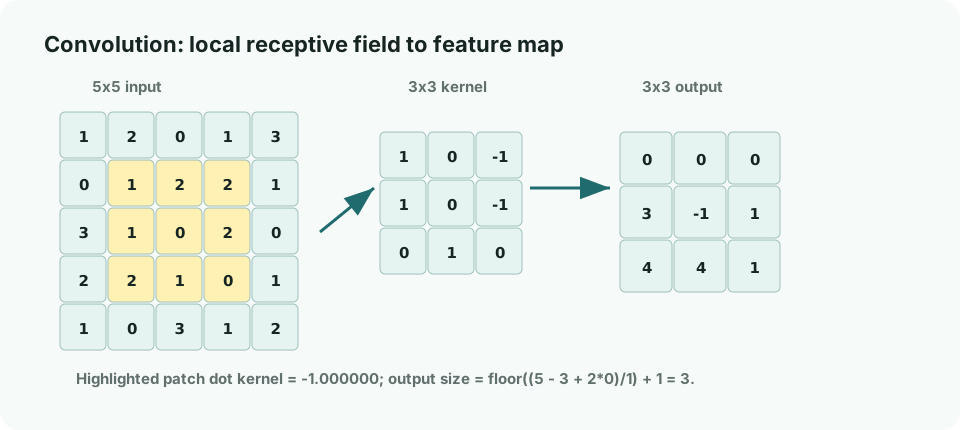
Input                         Kernel
[[1, 2, 0, 1, 3],             [[1, 0, -1],
 [0, 1, 2, 2, 1],              [1, 0, -1],
 [3, 1, 0, 2, 0],              [0, 1,  0]]
 [2, 2, 1, 0, 1],
 [1, 0, 3, 1, 2]]

Center patch                  Elementwise products
[[1, 2, 2],                   [[1, 0, -2],
 [1, 0, 2],                    [1, 0, -2],
 [2, 1, 0]]                    [0, 1,  0]]

Output
[[0,  0, 0],
 [3, -1, 1],
 [4,  4, 1]]
The center sum is 1 + 0 - 2 + 1 + 0 - 2 + 0 + 1 + 0 = -1. Output coordinates are zero-based, so this is row 1, column 1. The same patch is row 4 of a row-major im2col matrix because 1 * output_width + 1 = 4.
Complete runnable im2col example
import numpy as np


def conv2d_im2col(image, kernel, stride=1):
    """Single-channel valid cross-correlation, with no kernel flip."""
    image, kernel = (np.asarray(a, dtype=np.float64) for a in (image, kernel))
    if image.ndim != 2 or kernel.ndim != 2 or 0 in image.shape or 0 in kernel.shape:
        raise ValueError("nonempty two-dimensional arrays required")
    if not np.isfinite(image).all() or not np.isfinite(kernel).all():
        raise ValueError("finite inputs required")
    if isinstance(stride, (bool, np.bool_)) or not isinstance(stride, (int, np.integer)) or stride < 1:
        raise ValueError("stride must be a positive integer")
    h, w = image.shape
    kh, kw = kernel.shape
    if kh > h or kw > w:
        raise ValueError("kernel must fit the input")
    out_h, out_w = (h - kh) // stride + 1, (w - kw) // stride + 1
    cols = np.stack([
        image[r:r + kh, c:c + kw].reshape(-1)
        for r in range(0, h - kh + 1, stride)
        for c in range(0, w - kw + 1, stride)
    ])
    return (cols @ kernel.reshape(-1)).reshape(out_h, out_w)


image = np.array([[1, 2, 0, 1, 3],
                  [0, 1, 2, 2, 1],
                  [3, 1, 0, 2, 0],
                  [2, 2, 1, 0, 1],
                  [1, 0, 3, 1, 2]], dtype=np.float64)
kernel = np.array([[1, 0, -1], [1, 0, -1], [0, 1, 0]], dtype=np.float64)

if __name__ == "__main__":
    output = conv2d_im2col(image, kernel)
    print("Output shape:", output.shape)
    print(output)
    print("Center:", output[1, 1])
The minimal program performs valid, single-channel correlation. The extended conv_core.py adds zero padding and dilation; neither program is a complete neural-network layer. Both use float64. The im2col matrix has shape (9,9): one row per output location, nine entries per flattened patch.
4. Negative Controls That Expose Hidden Mistakes
| Calculation | Center |
|---|---|
| Current image and unflipped kernel | -1 |
| Same image, kernel flipped on both axes | +1 |
| Old code: arange(25) and all-ones kernel | 108 |
The old code’s 108 is the sum of a different patch, not rounding error around -1. Keeping it as a negative control makes the original mismatch reproducible. A further test flattens the kernel in column-major order while leaving image patches row-major; it produces a maximum absolute output error of 6. Shape checks alone do not detect that ordering mistake.
For new implementations, test a non-square image, a non-square kernel and an asymmetric kernel before trying a large model. The extended lab also checks a reversed input view with negative strides and confirms that neither input array is modified.
5. Executed Tests, Not Just a Checklist
The reference run used Python 3.13.9 and NumPy 2.3.5 on CPU. An independent scalar oracle computes source coordinates directly, without NumPy padding, sliding windows, reshape or matrix multiplication. With seed 42, the audit tried 640 candidate geometries: 512 with small integer entries and 128 with normally distributed entries.
| Check | Result |
|---|---|
| Valid generated geometries | 501 passed |
| Effective kernel too large | 139 rejected |
| Maximum numerical error | 3.6e-15 |
| Explicit malformed inputs | 12 rejected |
| RF coordinate comparisons | 18 passed |
Numerical comparisons use atol=1e-12 and rtol=1e-12. Invalid inputs include zero/fractional/boolean stride, zero dilation, negative or malformed padding, nonfinite values, empty arrays and an unexpected channel axis. These checks establish the stated small-array contract; they do not establish PyTorch parity, GPU speed or trained-model accuracy. Full values and source hashes are in audit.json.
6. Receptive-Field Span Is Not Uniform Influence
For a single sequential path, track three quantities along each axis: nominal receptive-field span r, the jump j between neighboring output centers in input coordinates, and the leftmost coordinate a for output zero. Initialize them to 1, 1 and 0.
a_new = a_old - pad_left * j_old
r_new = r_old + (kernel_size - 1) * dilation * j_old
j_new = j_old * stride
The order matters: use the previous jump when expanding the span. The Distill receptive-field derivation explains sequential paths, spatial alignment and the complications introduced by multiple branches.
| Successive layer | (r, j) |
|---|---|
| 3×3, stride 1, dilation 1 | (3, 1) |
| 3×3, stride 2, dilation 1 | (5, 2) |
| 3×3, stride 1, dilation 2 | (13, 2) |
The audit compares these recurrences with direct enumeration of possible input positions. A single dilated three-tap filter visits positions 0, 2 and 4: its nominal span is five, but it has holes. Padding shifts coordinates and may place part of the nominal box outside the real image. A size alone therefore does not identify every contributing pixel.
Now consider a separate, fully specified sensitivity experiment: a 5-by-5 input, two valid 3-by-3 all-ones filters, stride 1, and no bias or activation. The output is one scalar. Starting from zero input, add one to each input pixel individually and record the output change:

The matrix is the outer product of [1,2,3,2,1] with itself. Its corners are 1, its center is 9, and all coefficients sum to 81. An independent analytic check verifies all 25 measured coefficients. These results should not be confused with the effective receptive field studied in Luo and colleagues’ paper, which concerns how influence is distributed within theoretical support in deeper networks.
7. Measure the Explicit Patch Matrix, Not an Imagined GPU Benchmark
| Our float64 fixture | Bytes |
|---|---|
| 5×5 input array | 200 |
| 9×9 explicit im2col matrix | 648 |
| 3×3 output array | 72 |
These are actual NumPy nbytes values, not peak process memory. Padding, reshape/materialization temporaries, Python objects and allocator overhead are additional. The patch matrix alone is 3.24 times the input payload for this small valid example.
For an illustrative batch-1, 64-channel, 224-by-224 float32 input and a stride-one, padding-one 3-by-3 operation, the input payload is 12.25 MiB and an explicitly materialized patch matrix is 110.25 MiB. The script computes those sizes without allocating them. This is not an OOM observation or a speed measurement.
Do not conclude that every framework allocates that matrix. NVIDIA’s convolution guide distinguishes implicit GEMM from explicit materialization and also describes transform-based algorithms. The selected implementation depends on the backend and configuration. Choosing a padding mode is similarly a modeling decision: zero is not universally a black pixel after normalization, and reflection is not guaranteed to improve accuracy.
8. Reproduce, Then Extend One Variable at a Time
Extract the lab ZIP and run in its directory:
python3 -m venv .venv
source .venv/bin/activate
python -m pip install -r requirements.txt
python conv_example.py
python audit_convolution.py --out results
Success ends with CONVOLUTION_AUDIT_OK. The output directory does not overwrite the packaged reference. To regenerate the sensitivity figure, install requirements-plot.txt and run plot_sensitivity.py. CSVs retain full displayed float precision; compare using the documented tolerances across platforms.
Two useful exercises have known answers: use dilation 2 on the original fixture and obtain a 1-by-1 output equal to 4; then use padding 1 and obtain a 5-by-5 output whose top-left value is -2. Investigate one change at a time before adding channels, groups, nonlinearities or a new backend.
Continue with the Attention and KV cache experiment. Its analogous failure is not kernel orientation but query/key visibility: a correctly shaped tensor can still describe the wrong computation.