English
Gradient Descent and Optimizer Geometry: Momentum, Adam, and Loss Surfaces
An optimizer decides how parameters move along gradients. To understand gradient descent, momentum, and Adam, it is better to watch their paths on a loss surface than to memorize names. By exploring the geometry of optimization, we can understand why neural networks train efficiently or fail spectacularly.
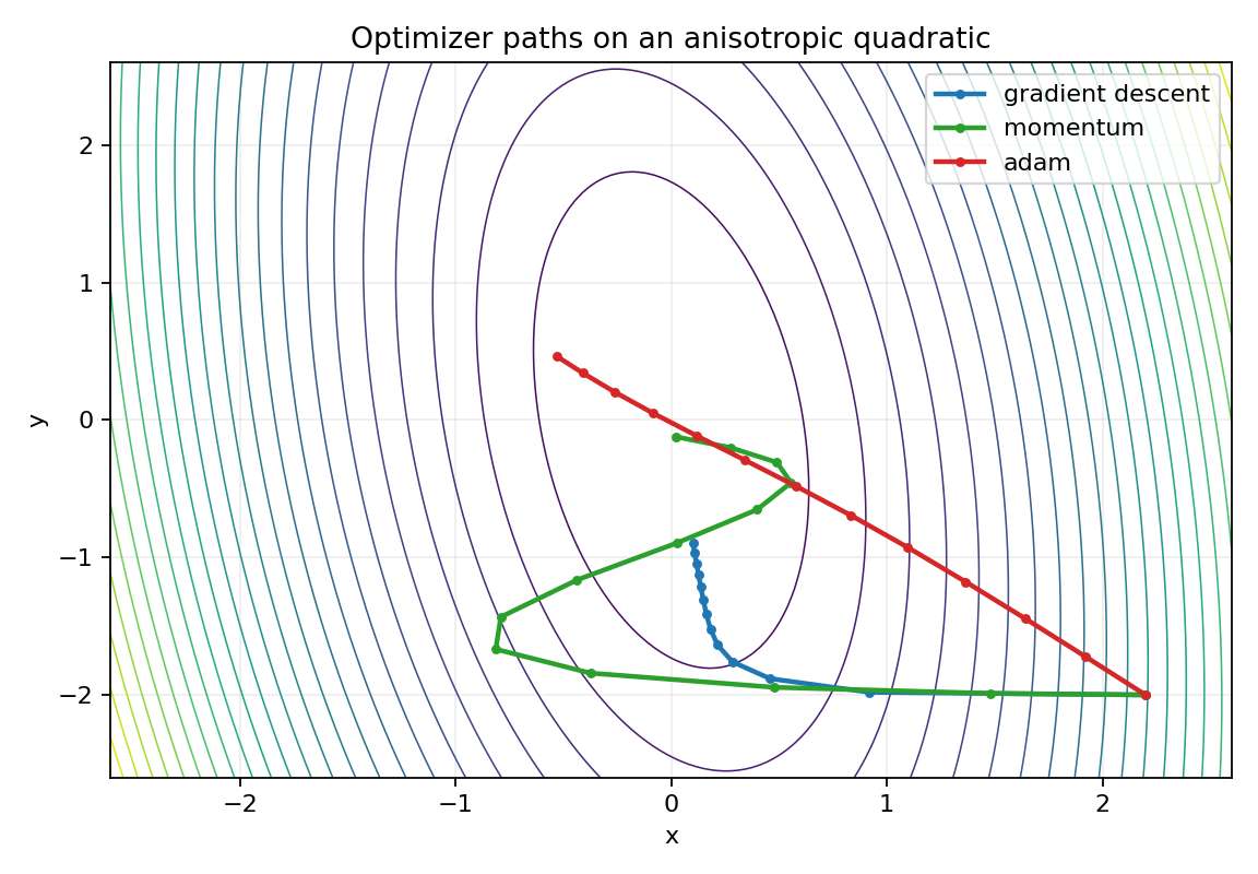
This article uses a two-dimensional quadratic function. The start point and target are the same, but different optimizers take completely different routes because they treat curvature, history, and scale differently. We will delve into the mathematical underpinnings and the real-world engineering constraints of these algorithms.
1. The Geometry of the Loss Surface and Pathological Curvature
In deep learning, the loss surface is rarely isotropic (perfectly spherical). Instead, it is highly ill-conditioned, filled with ravines and narrow valleys. Let's look at a canonical function demonstrating this:
L(x, y) = 1/2 * (8x^2 + y^2) + 0.8xy
grad L = [8x + 0.8y, y + 0.8x]
The Hessian matrix of this function has disparate eigenvalues. The surface is steep in the x direction (high curvature) and flatter in the y direction (low curvature). This creates a "pathological curvature" problem. A plain Gradient Descent step will bounce back and forth across the steep ravine, making excruciatingly slow progress along the flat bottom towards the minimum.
2. Hand Calculate The First Gradient Descent Step
Starting from (2.2, -2.0), the gradient is:
grad = [8*2.2 + 0.8*(-2.0), -2.0 + 0.8*2.2]
= [16.0, -0.24]
With a learning rate of 0.08:
x_new = 2.2 - 0.08 * 16.0 = 0.92
y_new = -2.0 - 0.08 * -0.24 = -1.9808
The step taken in the x direction is massive compared to y, purely because the gradient is overwhelmingly larger in x. The lab output confirms it: step 1 for gradient descent is x=0.920000, y=-1.980800, and the loss drops from 17.840000 to 3.889516. However, if the learning rate were just slightly higher, the step in x would overshoot the valley, leading to divergence.
3. What Momentum And Adam Change
Plain gradient descent is memoryless; it only uses the current gradient. This leads to the aforementioned oscillation.
Momentum accumulates a velocity from previous gradients. Think of a heavy ball rolling down a hill. The alternating gradients in the steep x direction cancel each other out, while the consistent gradients in the flat y direction accumulate, accelerating the optimizer toward the minimum.
v_t = beta * v_{t-1} + grad_t
theta_t = theta_{t-1} - lr * v_t
Adam (Adaptive Moment Estimation) goes a step further by maintaining both first (mean) and second (uncentered variance) moments of the gradients. It dynamically scales the learning rate for each parameter individually. By dividing the update by the square root of the accumulated squared gradients, Adam normalizes the step sizes. It essentially forces the optimizer to take larger steps in flat directions and smaller steps in steep directions.
m_t = beta1 * m_{t-1} + (1-beta1) * grad_t
v_t = beta2 * v_{t-1} + (1-beta2) * grad_t^2
theta_t = theta_{t-1} - lr * m_hat / (sqrt(v_hat) + eps)
4. Optimizer Anatomy: Visualized
How do we decide which optimizer to use? The diagram below visualizes the architectural flow of these optimization algorithms.
graph TD
A[Compute Gradient] --> B{Need history?}
B -->|No| C[Vanilla SGD]
B -->|Yes| D{Adaptive Scale?}
D -->|No| E[SGD with Momentum]
D -->|Yes| F[Compute 1st & 2nd Moments]
F --> G[Bias Correction]
G --> H[Adam / AdamW]
C --> I[Apply Parameter Update]
E --> I
H --> I
5. Practical Python Implementation
To truly grasp these algorithms, we should build them from scratch. Here is a NumPy implementation comparing SGD, Momentum, and Adam on our quadratic surface.
import numpy as np
def grad(theta):
x, y = theta
return np.array([8.0 * x + 0.8 * y, y + 0.8 * x])
def run_optimizer(optimizer_name, theta_init, lr=0.08, steps=50):
theta = np.array(theta_init)
# Optimizer state
v = np.zeros_like(theta)
m = np.zeros_like(theta)
beta1, beta2, eps = 0.9, 0.999, 1e-8
trajectory = [theta.copy()]
for t in range(1, steps + 1):
g = grad(theta)
if optimizer_name == 'SGD':
theta -= lr * g
elif optimizer_name == 'Momentum':
v = 0.9 * v + lr * g
theta -= v
elif optimizer_name == 'Adam':
m = beta1 * m + (1 - beta1) * g
v = beta2 * v + (1 - beta2) * (g ** 2)
# Bias correction
m_hat = m / (1 - beta1 ** t)
v_hat = v / (1 - beta2 ** t)
theta -= lr * m_hat / (np.sqrt(v_hat) + eps)
trajectory.append(theta.copy())
return np.array(trajectory)
# Run test from the start point
traj_sgd = run_optimizer('SGD', [2.2, -2.0])
traj_adam = run_optimizer('Adam', [2.2, -2.0], lr=0.5)
print(f"Final Adam position: {traj_adam[-1]}")
6. What The Animation Shows
Watch whether the steep direction oscillates and whether the flatter direction progresses too slowly. Notice how Momentum swings widely like a pendulum before settling, while Adam cuts a much more direct, controlled path toward the minimum, seamlessly adjusting to the varying curvature.
7. Personal Experience / Engineer's Perspective
In practice, the elegant math of optimizers runs into harsh hardware and systems realities. Here are a few things I've learned from the trenches of training large models:
- Memory Constraints: Adam is highly effective but extremely memory-hungry. Vanilla SGD only requires memory for the parameters and gradients. Adam requires storing the moving average of gradients (first moment) and the moving average of squared gradients (second moment). This essentially triples the memory footprint of your optimizer state. When training large LLMs on GPUs with limited VRAM, this is often the bottleneck, prompting engineers to use memory-efficient variants like Adafactor or 8-bit Adam.
- Weight Decay Pitfalls: There is a notorious difference between Adam and AdamW. Standard Adam applies L2 regularization to the gradient before the adaptive scaling. This inadvertently scales down the penalty for weights with high gradient variance, defeating the purpose of weight decay. Always use AdamW for Transformer architectures, which decouples weight decay from the gradient update.
- Warmup is Mandatory for Adam: Because Adam uses moving averages, the variance term (second moment) is initialized to zero and can be wildly inaccurate in the first few steps, leading to massive, destabilizing updates. A learning rate warmup (starting the LR near zero and scaling up over thousands of steps) prevents the model from blowing up early in training.
8. Practical Notes
- Plot training and validation loss before changing optimizers. Many training failures are optimizer-path problems rather than architecture problems.
- The learning rate usually matters more than the optimizer name. A well-tuned SGD with Momentum can often match or beat Adam in generalization, especially in computer vision (ResNets).
- Adam can still diverge when the learning rate is too high. Do not treat it as a silver bullet that requires no tuning.
- For noisy loss curves, try lowering the learning rate or adding warmup.
9. Optimization Trace Audit Table
An optimizer experiment should not report only the final loss. To judge whether the path is trustworthy, record coordinates, gradients, state variables, and failure modes together. The audit table below turns "it seems to converge" into reproducible numerical evidence.
| Audit item | Values to record | Question it answers |
|---|---|---|
| Initial condition | Start point, learning rate, step count, and optimizer hyperparameters. | Are the curves being compared under the same conditions? |
| Step trace | x, y, loss, gradient vector, and update size. |
Is the path descending, or bouncing across the ravine? |
| State variables | Momentum v; Adam m, v, and bias correction. |
Did history and adaptive scaling actually change the path? |
| Failure mode | Divergent step, oscillation band, oversized early update, and final distance. | Does failure come from learning rate, curvature, initialization, or optimizer state? |
The next article moves into convolution and shows how local image operations become matrix computations.
Chinese
梯度下降与优化器几何:Momentum、Adam 和 loss surface 轨迹
Open as a full page优化器决定了模型参数如何沿着梯度方向移动。要真正理解梯度下降(Gradient Descent)、动量(Momentum)和 Adam,不要仅仅死记硬背它们的名字或公式,而是要观察它们在损失函数曲面(Loss Surface)上走出的轨迹。通过探索优化的几何学,我们可以理解为什么神经网络有时能高效训练,有时却会面临灾难性的失败。
这篇文章使用了一个二维二次函数来进行可视化分析。虽然起点和目标相同,但不同的优化器会因为对曲率、历史梯度和尺度的处理方式不同,从而走出截然不同的路线。我们将深入探讨这些算法背后的数学原理以及现实工程中的约束。
一、损失曲面的几何与病态曲率
在深度学习中,损失曲面极少是各向同性的(即完美的球形)。相反,它通常是高度病态的,充满了峡谷和狭长的山谷。让我们来看一个典型的用来演示这个问题的函数:
L(x, y) = 1/2 * (8x^2 + y^2) + 0.8xy
grad L = [8x + 0.8y, y + 0.8x]
这个函数的 Hessian 矩阵具有差异极大的特征值。该曲面在 x 方向非常陡峭(高曲率),而在 y 方向则较为平缓(低曲率)。这就造成了所谓的“病态曲率(Pathological Curvature)”问题。普通的梯度下降算法会在陡峭的峡谷两侧来回震荡,而在通向极小值的平缓谷底方向上进展极其缓慢。
二、手算第一步梯度下降
从 (2.2, -2.0) 出发,梯度为:
grad = [8*2.2 + 0.8*(-2.0), -2.0 + 0.8*2.2]
= [16.0, -0.24]
如果学习率是 0.08:
x_new = 2.2 - 0.08 * 16.0 = 0.92
y_new = -2.0 - 0.08 * -0.24 = -1.9808
与 y 方向相比,参数在 x 方向上迈出了一大步,这纯粹是因为 x 方向的梯度绝对值大得多。实验输出也印证了这一点:梯度下降第 1 步的坐标是 x=0.920000、y=-1.980800,loss 从 17.840000 降到了 3.889516。然而,如果学习率稍微再大一点,x 方向的步长就会跨过山谷的另一端,导致发散。
三、Momentum 和 Adam 在改什么
普通梯度下降是没有记忆的;它只看当前的梯度。这正是导致上述震荡的原因。
动量(Momentum) 引入了速度变量,把过去的梯度方向累积起来。想象一个沉重的球滚下山坡。在陡峭的 x 方向上,交替正负的梯度会相互抵消;而在平缓的 y 方向上,方向一致的梯度不断累加,从而加速优化器冲向极小值。
v_t = beta * v_{t-1} + grad_t
theta_t = theta_{t-1} - lr * v_t
Adam(Adaptive Moment Estimation) 则更进一步,它同时维护梯度的一阶矩(均值)和二阶矩(未中心化的方差)。它能够为每一个参数单独动态缩放学习率。通过除以累积梯度平方的平方根,Adam 归一化了步长。它本质上是强迫优化器在平缓的方向迈大步,在陡峭的方向迈小步。
m_t = beta1 * m_{t-1} + (1-beta1) * grad_t
v_t = beta2 * v_{t-1} + (1-beta2) * grad_t^2
theta_t = theta_{t-1} - lr * m_hat / (sqrt(v_hat) + eps)
四、优化器决策流程图解
我们该如何决定使用哪种优化器?下面的图表直观地展示了这些优化算法的架构流程。
graph TD
A[计算当前梯度] --> B{是否需要历史信息?}
B -->|否| C[普通 SGD]
B -->|是| D{是否需要自适应缩放?}
D -->|否| E[带 Momentum 的 SGD]
D -->|是| F[计算一阶和二阶矩]
F --> G[偏差修正]
G --> H[Adam / AdamW]
C --> I[应用参数更新]
E --> I
H --> I
五、核心代码实践与实现
为了真正掌握这些算法,我们应该从零开始构建它们。以下是使用 NumPy 在我们的二次曲面上对比 SGD、Momentum 和 Adam 的核心实现。
import numpy as np
def grad(theta):
x, y = theta
return np.array([8.0 * x + 0.8 * y, y + 0.8 * x])
def run_optimizer(optimizer_name, theta_init, lr=0.08, steps=50):
theta = np.array(theta_init)
# 初始化优化器状态
v = np.zeros_like(theta)
m = np.zeros_like(theta)
beta1, beta2, eps = 0.9, 0.999, 1e-8
trajectory = [theta.copy()]
for t in range(1, steps + 1):
g = grad(theta)
if optimizer_name == 'SGD':
theta -= lr * g
elif optimizer_name == 'Momentum':
v = 0.9 * v + lr * g
theta -= v
elif optimizer_name == 'Adam':
m = beta1 * m + (1 - beta1) * g
v = beta2 * v + (1 - beta2) * (g ** 2)
# 偏差修正
m_hat = m / (1 - beta1 ** t)
v_hat = v / (1 - beta2 ** t)
theta -= lr * m_hat / (np.sqrt(v_hat) + eps)
trajectory.append(theta.copy())
return np.array(trajectory)
# 从起点运行测试
traj_sgd = run_optimizer('SGD', [2.2, -2.0])
traj_adam = run_optimizer('Adam', [2.2, -2.0], lr=0.5)
print(f"Adam 最终位置: {traj_adam[-1]}")
六、动画看什么
重点看两点:陡峭方向上是否震荡,平缓方向上是否前进太慢。注意 Momentum 是如何像钟摆一样大幅度摇摆才最终稳定下来的,而 Adam 则是切出了一条更加直接、可控的路径,完美适应了不断变化的曲率。
七、个人经验与工程师视角
在工程实践中,优化器优雅的数学原理往往会撞上残酷的硬件和系统现实。以下是我在训练大模型时积累的一些经验:
- 显存(Memory)瓶颈: Adam 效果极好,但极其消耗显存。普通的 SGD 只需要为参数和梯度分配显存。而 Adam 还需要存储梯度的滑动平均(一阶矩)和梯度平方的滑动平均(二阶矩)。这使得优化器状态的显存占用直接翻了三倍。在显存受限的 GPU 上训练大型 LLM 时,这往往成为最大瓶颈,迫使工程师转向 Adafactor 或 8-bit Adam 等显存友好型变体。
- 权重衰减(Weight Decay)的陷阱: Adam 和 AdamW 之间有着臭名昭著的区别。标准的 Adam 在自适应缩放之前对梯度应用 L2 正则化。这无意中削弱了对梯度方差较大的权重的惩罚力度,违背了权重衰减的初衷。对于 Transformer 架构,一定要使用 AdamW,它将权重衰减与梯度更新步骤完全解耦。
- Adam 必须配合 Warmup 使用: 因为 Adam 使用了滑动平均,方差项(二阶矩)初始为零,在最初的几步中可能会极其不准确,导致出现极其巨大且破坏性的更新。引入学习率预热(Warmup,即让学习率从接近零开始,在几千步内逐渐攀升)可以防止模型在训练初期直接崩溃。
八、实践建议
- 先画训练 loss 和验证 loss,再判断是否需要换优化器。很多训练问题其实是优化路径不稳定,而不是模型结构错了。
- 学习率通常比优化器的名称更关键。一个经过精心调参的带 Momentum 的 SGD,其泛化能力通常能媲美甚至超越 Adam,尤其是在计算机视觉领域(如 ResNet)。
- Adam 并非万能药,过大的学习率仍然会导致它发散。
- 遇到 loss 曲线抖动时,先尝试降低学习率或加 warmup。
九、优化轨迹审计表
优化器实验不能只报告最终 loss。为了判断路径是否可信,应该同时记录坐标、梯度、状态变量和失败模式。下面的审计表可以帮助读者把“看起来收敛了”拆成可复核的数值证据。
| 审计项 | 应记录的值 | 能回答的问题 |
|---|---|---|
| 初始条件 | 起点、学习率、步数、优化器超参数。 | 不同曲线是否在同一条件下比较? |
| 逐步轨迹 | x、y、loss、梯度向量和步长。 |
路径是在下降,还是在峡谷两侧震荡? |
| 状态变量 | Momentum 的 v,Adam 的 m、v 和 bias correction。 |
历史梯度和自适应缩放是否真的改变了路径? |
| 失败模式 | 发散步、震荡区间、过大 warmup 前更新和最终距离。 | 失败来自学习率、曲率、初始化还是优化器状态? |
下一篇进入卷积层,看看二维局部连接如何变成矩阵计算。
An optimizer decides how parameters move along gradients. To understand gradient descent, momentum, and Adam, it is better to watch their paths on a loss surface than to memorize names. By exploring the geometry of optimization, we can understand why neural networks train efficiently or fail spectacularly.
This article uses a two-dimensional quadratic function. The start point and target are the same, but different optimizers take completely different routes because they treat curvature, history, and scale differently. We will delve into the mathematical underpinnings and the real-world engineering constraints of these algorithms.
1. The Geometry of the Loss Surface and Pathological Curvature
In deep learning, the loss surface is rarely isotropic (perfectly spherical). Instead, it is highly ill-conditioned, filled with ravines and narrow valleys. Let’s look at a canonical function demonstrating this:
L(x, y) = 1/2 * (8x^2 + y^2) + 0.8xy
grad L = [8x + 0.8y, y + 0.8x]
The Hessian matrix of this function has disparate eigenvalues. The surface is steep in the x direction (high curvature) and flatter in the y direction (low curvature). This creates a “pathological curvature” problem. A plain Gradient Descent step will bounce back and forth across the steep ravine, making excruciatingly slow progress along the flat bottom towards the minimum.

2. Hand Calculate The First Gradient Descent Step
Starting from (2.2, -2.0), the gradient is:
grad = [8*2.2 + 0.8*(-2.0), -2.0 + 0.8*2.2]
= [16.0, -0.24]
With a learning rate of 0.08:
x_new = 2.2 - 0.08 * 16.0 = 0.92
y_new = -2.0 - 0.08 * -0.24 = -1.9808
The step taken in the x direction is massive compared to y, purely because the gradient is overwhelmingly larger in x. The lab output confirms it: step 1 for gradient descent is x=0.920000, y=-1.980800, and the loss drops from 17.840000 to 3.889516. However, if the learning rate were just slightly higher, the step in x would overshoot the valley, leading to divergence.
3. What Momentum And Adam Change
Plain gradient descent is memoryless; it only uses the current gradient. This leads to the aforementioned oscillation.
Momentum accumulates a velocity from previous gradients. Think of a heavy ball rolling down a hill. The alternating gradients in the steep x direction cancel each other out, while the consistent gradients in the flat y direction accumulate, accelerating the optimizer toward the minimum.
v_t = beta * v_{t-1} + grad_t
theta_t = theta_{t-1} - lr * v_t
Adam (Adaptive Moment Estimation) goes a step further by maintaining both first (mean) and second (uncentered variance) moments of the gradients. It dynamically scales the learning rate for each parameter individually. By dividing the update by the square root of the accumulated squared gradients, Adam normalizes the step sizes. It essentially forces the optimizer to take larger steps in flat directions and smaller steps in steep directions.
m_t = beta1 * m_{t-1} + (1-beta1) * grad_t
v_t = beta2 * v_{t-1} + (1-beta2) * grad_t^2
theta_t = theta_{t-1} - lr * m_hat / (sqrt(v_hat) + eps)
4. Optimizer Anatomy: Visualized
How do we decide which optimizer to use? The diagram below visualizes the architectural flow of these optimization algorithms.
graph TD
A[Compute Gradient] --> B{Need history?}
B -->|No| C[Vanilla SGD]
B -->|Yes| D{Adaptive Scale?}
D -->|No| E[SGD with Momentum]
D -->|Yes| F[Compute 1st & 2nd Moments]
F --> G[Bias Correction]
G --> H[Adam / AdamW]
C --> I[Apply Parameter Update]
E --> I
H --> I
5. Practical Python Implementation
To truly grasp these algorithms, we should build them from scratch. Here is a NumPy implementation comparing SGD, Momentum, and Adam on our quadratic surface.
import numpy as np
def grad(theta):
x, y = theta
return np.array([8.0 * x + 0.8 * y, y + 0.8 * x])
def run_optimizer(optimizer_name, theta_init, lr=0.08, steps=50):
theta = np.array(theta_init)
# Optimizer state
v = np.zeros_like(theta)
m = np.zeros_like(theta)
beta1, beta2, eps = 0.9, 0.999, 1e-8
trajectory = [theta.copy()]
for t in range(1, steps + 1):
g = grad(theta)
if optimizer_name == 'SGD':
theta -= lr * g
elif optimizer_name == 'Momentum':
v = 0.9 * v + lr * g
theta -= v
elif optimizer_name == 'Adam':
m = beta1 * m + (1 - beta1) * g
v = beta2 * v + (1 - beta2) * (g ** 2)
# Bias correction
m_hat = m / (1 - beta1 ** t)
v_hat = v / (1 - beta2 ** t)
theta -= lr * m_hat / (np.sqrt(v_hat) + eps)
trajectory.append(theta.copy())
return np.array(trajectory)
# Run test from the start point
traj_sgd = run_optimizer('SGD', [2.2, -2.0])
traj_adam = run_optimizer('Adam', [2.2, -2.0], lr=0.5)
print(f"Final Adam position: {traj_adam[-1]}")
6. What The Animation Shows
Watch whether the steep direction oscillates and whether the flatter direction progresses too slowly. Notice how Momentum swings widely like a pendulum before settling, while Adam cuts a much more direct, controlled path toward the minimum, seamlessly adjusting to the varying curvature.
7. Personal Experience / Engineer’s Perspective
In practice, the elegant math of optimizers runs into harsh hardware and systems realities. Here are a few things I’ve learned from the trenches of training large models:
- Memory Constraints: Adam is highly effective but extremely memory-hungry. Vanilla SGD only requires memory for the parameters and gradients. Adam requires storing the moving average of gradients (first moment) and the moving average of squared gradients (second moment). This essentially triples the memory footprint of your optimizer state. When training large LLMs on GPUs with limited VRAM, this is often the bottleneck, prompting engineers to use memory-efficient variants like Adafactor or 8-bit Adam.
- Weight Decay Pitfalls: There is a notorious difference between Adam and AdamW. Standard Adam applies L2 regularization to the gradient before the adaptive scaling. This inadvertently scales down the penalty for weights with high gradient variance, defeating the purpose of weight decay. Always use AdamW for Transformer architectures, which decouples weight decay from the gradient update.
- Warmup is Mandatory for Adam: Because Adam uses moving averages, the variance term (second moment) is initialized to zero and can be wildly inaccurate in the first few steps, leading to massive, destabilizing updates. A learning rate warmup (starting the LR near zero and scaling up over thousands of steps) prevents the model from blowing up early in training.
8. Practical Notes
- Plot training and validation loss before changing optimizers. Many training failures are optimizer-path problems rather than architecture problems.
- The learning rate usually matters more than the optimizer name. A well-tuned SGD with Momentum can often match or beat Adam in generalization, especially in computer vision (ResNets).
- Adam can still diverge when the learning rate is too high. Do not treat it as a silver bullet that requires no tuning.
- For noisy loss curves, try lowering the learning rate or adding warmup.
9. Optimization Trace Audit Table
An optimizer experiment should not report only the final loss. To judge whether the path is trustworthy, record coordinates, gradients, state variables, and failure modes together. The audit table below turns “it seems to converge” into reproducible numerical evidence.
| Audit item | Values to record | Question it answers |
|---|---|---|
| Initial condition | Start point, learning rate, step count, and optimizer hyperparameters. | Are the curves being compared under the same conditions? |
| Step trace | x, y, loss, gradient vector, and update size. |
Is the path descending, or bouncing across the ravine? |
| State variables | Momentum v; Adam m, v, and bias correction. |
Did history and adaptive scaling actually change the path? |
| Failure mode | Divergent step, oscillation band, oversized early update, and final distance. | Does failure come from learning rate, curvature, initialization, or optimizer state? |
The next article moves into convolution and shows how local image operations become matrix computations.
Search questions
FAQ
Who is this article for?
This article is for readers who want an intermediate-level guide to Gradient Descent and Optimizer Geometry. It takes about 13 min and focuses on Gradient Descent, Momentum, Adam, Loss Surface.
What should I read next?
The recommended next step is Convolution and Receptive Field Math, so the article connects into a longer learning route instead of ending as an isolated note.
Does this article include runnable code or companion resources?
Yes. Use the run notes, resource cards, and download links on the page to reproduce the example or inspect the companion files.
How does this article fit into the larger site?
It is connected to the article context block, learning routes, resources, and project timeline so readers can move from concept to implementation.
Article context
AI Learning Project
A practical route from AI concepts to machine learning workflow, evaluation, neural networks, Python practice, handwritten digits, a CIFAR-10 CNN, adversarial traffic-defense notes, and AI security.
Compare gradient descent, momentum, and Adam on a visible quadratic loss surface.
Download share card Open share centerCompanion resources
AI Learning Project / DATASET
Optimizer path CSV
Step-by-step coordinates and loss for gradient descent, momentum, and Adam on a 2D quadratic.
AI Learning Project / TOOL
Deep learning math interactive visualizer
Browser modules for gradient checking, optimizer paths, convolution output size, and attention heatmaps.
AI Learning Project / ARCHIVE
Deep learning math full lab bundle
Bundles NumPy scripts, CSV outputs, formula diagrams, loss contours, convolution figures, and attention heatmaps.
Project timeline
Published posts
- AI Basics Learning Roadmap Separate AI, machine learning, and deep learning before going into implementation details.
- Machine Learning Workflow Follow the practical path from data and features to training, prediction, and evaluation.
- Model Training and Evaluation Understand loss, overfitting, train/test splits, accuracy, recall, and F1.
- Neural Network Basics Move from perceptrons to activation, forward propagation, backpropagation, and training loops.
- Matrix Calculus for Neural Networks Derive dL/dW for y = Wx + b and verify it with finite differences.
- Backpropagation as a Computation Graph Trace local gradients through ReLU and softmax cross-entropy in a two-layer MLP.
- Gradient Descent and Optimizer Geometry Compare gradient descent, momentum, and Adam on a visible quadratic loss surface.
- Convolution and Receptive Field Math Compute convolution output size, receptive fields, channel mixing, and im2col layout.
- Transformer Attention Math Hand-calculate Q/K/V scores, softmax weights, masks, multi-head structure, and KV cache.
- Python AI Mini Practice Run a small scikit-learn classification task and read the experiment output.
- Handwritten Digit Dataset Basics Read train.csv, test.csv, labels, and the flattened 28 by 28 pixel layout before training the classifier.
- Handwritten Digit Softmax in C Follow the C implementation from logits and softmax probabilities to confusion matrices and submission export.
- Handwritten Digit Playground Notes See how the offline classifier was adapted into a browser demo with drawing input and probability output.
- CIFAR-10 Tiny CNN Tutorial in C Build and train a small convolutional neural network for CIFAR-10 image classification, then read its loss and accuracy output.
- High-Entropy Traffic Defense Notes Study encrypted metadata leaks, entropy, traffic classifiers, and a defensive Python chaffing prototype.
- AI Security Threat Modeling Build a defense map with NIST adversarial ML, MITRE ATLAS, and OWASP LLM risks.
- Adversarial Examples and Robust Evaluation Evaluate clean and perturbed accuracy with an FGSM-style digits experiment.
- Data Poisoning and Backdoor Defense Study poison rate, trigger behavior, attack success rate, and training pipeline controls.
- Model Privacy and Extraction Defense Measure membership inference signal and surrogate fidelity against a local toy model.
- LLM, RAG, and Agent Security Separate instructions from data and enforce tool permissions against indirect prompt injection.
Published resources
- Python AI practice code guide The article includes a runnable scikit-learn classification script.
- digit_softmax_classifier.c The C source for the handwritten digit softmax classifier.
- train.csv.zip Compressed handwritten digit training set with 42000 labeled samples.
- test.csv.zip Compressed handwritten digit test set with 28000 unlabeled samples.
- sample_submission.csv The official submission format example for checking the final output columns.
- submission.csv The prediction file generated by the current C project.
- digit-playground-model.json The compact softmax demo model and sample set used by the browser playground.
- digit-sample-grid.svg A small handwritten digit preview grid extracted from the training set.
- Handwritten digit project bundle Contains the source file, compressed datasets, submission files, browser model, and preview grid.
- cifar10_tiny_cnn.c source Single-file C tiny CNN with CIFAR-10 loading, convolution, pooling, softmax, and backpropagation.
- model_weights.bin sample weights Model weights generated by one local small-sample run.
- test_predictions.csv sample predictions Sample test prediction output from the CIFAR-10 tiny CNN.
- CNN project explanation PDF Companion explanation material for the CNN project.
- Virtual Mirror redacted code skeleton A redacted mld_chaffing_v2.py control-flow skeleton with secrets, node topology, and target lists removed.
- Virtual Mirror stress-test template A redacted CSV template for CPU, memory, peak threads, pulse rate, latency, and error measurements.
- Virtual Mirror classifier-evaluation template A CSV template for TP, FN, FP, TN, accuracy, precision, recall, F1, ROC-AUC, entropy, and JS divergence.
- Virtual Mirror resource notes Notes explaining why the public resources include only redacted code, test templates, and architecture context.
- AI Security Lab README Setup, safety boundaries, and quick-run commands for the AI Security series.
- AI Security Lab full bundle Includes safe toy scripts, result CSVs, risk register, attack-defense matrix, and architecture diagram.
- AI security risk register CSV risk register template for AI threat modeling and release review.
- AI attack-defense matrix Maps attack surface, toy demo, metric, and defensive control into one CSV table.
- AI Security Lab architecture diagram Shows threat modeling, robustness, data integrity, model privacy, and RAG guardrails.
- FGSM digits robustness script FGSM-style perturbation and accuracy-drop experiment for a local digits classifier.
- Data poisoning and backdoor toy script Demonstrates poison rate, trigger behavior, and attack success rate on digits.
- Model privacy and extraction toy script Outputs membership AUC, target accuracy, surrogate fidelity, and surrogate accuracy.
- RAG prompt injection guard toy script Uses a deterministic toy agent to demonstrate external-data demotion and tool-policy blocking.
- Deep Learning Math Lab README Setup commands, script entry points, generated outputs, and figure notes for the math series.
- Deep learning math full lab bundle Bundles NumPy scripts, CSV outputs, formula diagrams, loss contours, convolution figures, and attention heatmaps.
- Gradient check results CSV Stores MSE analytic gradients, finite-difference gradients, and error norms.
- Optimizer path CSV Step-by-step coordinates and loss for gradient descent, momentum, and Adam on a 2D quadratic.
- Attention weights CSV Scores, softmax weights, and context vectors for a three-token scaled dot-product attention example.
- Deep learning math figure set Includes matrix shapes, computation graphs, loss contours, convolution scans, and attention heatmaps.
- Deep learning math interactive visualizer Browser modules for gradient checking, optimizer paths, convolution output size, and attention heatmaps.
- Deep Learning topic share card A 1200x630 SVG card for sharing the Deep Learning / CNN topic hub.
- Machine Learning From Scratch share card A 1200x630 SVG card for the K-means, Iris, and ML workflow topic hub.
- Student AI Projects share card A 1200x630 SVG card for handwritten digits, C classifiers, and browser demos.
- CNN convolution scan animation An 8-second Remotion animation showing how a 3x3 convolution kernel scans an input and builds a feature map.
Current route
- AI Basics Learning Roadmap Learning path step
- Machine Learning Workflow Learning path step
- Model Training and Evaluation Learning path step
- Neural Network Basics Learning path step
- Matrix Calculus for Neural Networks Learning path step
- Backpropagation as a Computation Graph Learning path step
- Gradient Descent and Optimizer Geometry Learning path step
- Convolution and Receptive Field Math Learning path step
- Transformer Attention Math Learning path step
- LLM Visualizer Learning path step
- Python AI Mini Practice Learning path step
- Handwritten Digit Dataset Basics Learning path step
- Handwritten Digit Softmax in C Learning path step
- Handwritten Digit Playground Notes Learning path step
- CIFAR-10 Tiny CNN Tutorial in C Learning path step
- High-Entropy Traffic Defense Notes Learning path step
- AI Security Threat Modeling Learning path step
- Adversarial Examples and Robust Evaluation Learning path step
- Data Poisoning and Backdoor Defense Learning path step
- Model Privacy and Extraction Defense Learning path step
- LLM, RAG, and Agent Security Learning path step
Next notes
- Add more image-classification and error-analysis cases
- Turn common metrics into a quick reference
- Add more AI security defense experiment notes