Matrix Calculus for Neural Networks: Deriving the MSE Gradient

Matrix calculus in deep learning is often perceived as an abstract academic exercise, but it is fundamentally a practical tool. It is not about making notation look difficult; it is a rigorous method to verify tensor shapes, align gradient directions, and validate code correctness. Once you can confidently derive and implement the gradient of a simple linear layer y_hat = Wx + b, complex architectures like backpropagation, convolutional layers, and attention mechanisms become significantly more tractable and much easier to debug.

This article dives deep into the anatomy of a single linear layer paired with a mean squared error (MSE) loss. Our goal is to demystify the mathematical formulas, connect them directly to hand calculations, and finally translate them into runnable, deterministic NumPy code that bridges theory and practice.

1. The Foundation: Dimension and Shape Tracking

In matrix calculus, keeping track of dimensions is half the battle. Let’s define our variables:

• x: A 3 x 1 column vector (input features).
• W: A 2 x 3 weight matrix.
• b: A 2 x 1 bias vector.
• y: A 2 x 1 column vector (target labels).

The forward pass and loss function are defined as:

y_hat = W x + b
e     = y_hat - y
L     = 1/2 * e^T e

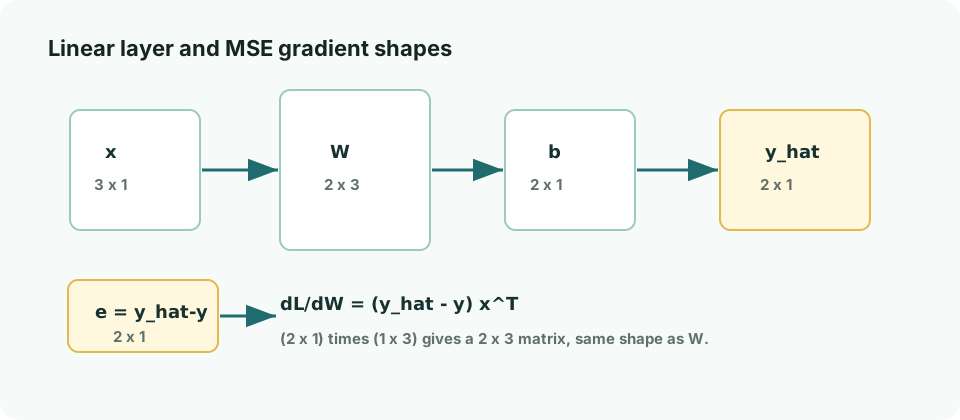
The most crucial habit to develop is shape checking at every step. The matrix multiplication W x yields a 2 x 1 vector. Consequently, the error vector e is also 2 x 1. A fundamental rule of matrix calculus states that the gradient of a scalar loss L with respect to a matrix W, denoted as dL/dW, must possess the exact same shape as W. Thus, dL/dW must be 2 x 3.

Visualizing the Forward and Backward Pass

To better conceptualize the flow of data and gradients, consider the following computational graph:

graph TD
    x[Input x: 3x1] --> Mul[Matrix Mul: W*x]
    W[Weights W: 2x3] --> Mul
    Mul --> Add[Add Bias: + b]
    b[Bias b: 2x1] --> Add
    Add --> y_hat[Prediction y_hat: 2x1]
    y_hat --> Error[Error e = y_hat - y]
    y[Target y: 2x1] --> Error
    Error --> Loss[Loss L = 1/2 * e^T * e]
    
    %% Backward pass
    Loss -.->|dL/de = e| Error
    Error -.->|dL/dW = e * x^T| W
    Error -.->|dL/db = e| b

2. Deriving the Gradient by Hand

Let’s calculate the analytical gradient. Starting with the loss function L = 1/2 * e^T e, the derivative with respect to the error vector is straightforward: dL/de = e.

Using the multivariate chain rule on e = Wx + b - y, we can derive the gradients for the parameters. The derivative of Wx with respect to W involves an outer product with the input transpose:

dL/dW = e x^T
dL/db = e

Let’s plug in some concrete numbers. Suppose the forward pass yields an error vector e = [0.2, 1.25]^T and our input was x = [1.5, -2.0, 0.5]^T. The gradient calculation becomes an outer product:

dL/dW =
[0.2 ] [ 1.5, -2.0, 0.5 ] = [ 0.300, -0.400, 0.100 ]
[1.25]                      [ 1.875, -2.500, 0.625 ]

This simple calculation is the bedrock of backpropagation. Every element W_{ij} is updated based on how much the j-th input feature contributed to the i-th output error.

3. Validating with Code: Numerical vs. Analytical Gradients

To trust our analytical derivation, we must verify it computationally using finite differences. Finite differences perturb one parameter at a time and estimate the loss slope from the change in loss, serving as a ground-truth check.

import numpy as np

def forward(W, b, x, y):
    y_hat = np.dot(W, x) + b
    e = y_hat - y
    loss = 0.5 * np.sum(e ** 2)
    return loss, e

def analytical_gradient(e, x):
    # Outer product: (2x1) * (1x3) -> (2x3)
    dW = np.dot(e, x.T)
    db = np.sum(e, axis=1, keepdims=True)
    return dW, db

def numeric_gradient_W(W, b, x, y, eps=1e-5):
    grad = np.zeros_like(W)
    for row in range(W.shape[0]):
        for col in range(W.shape[1]):
            original = W[row, col]
            
            W[row, col] = original + eps
            plus_loss, _ = forward(W, b, x, y)
            
            W[row, col] = original - eps
            minus_loss, _ = forward(W, b, x, y)
            
            W[row, col] = original # restore
            grad[row, col] = (plus_loss - minus_loss) / (2 * eps)
    return grad

# Setup dummy data
W = np.random.randn(2, 3)
b = np.random.randn(2, 1)
x = np.array([[1.5], [-2.0], [0.5]])
y = np.random.randn(2, 1)

# Compute
_, e = forward(W, b, x, y)
dW_analytical, db_analytical = analytical_gradient(e, x)
dW_numeric = numeric_gradient_W(W, b, x, y)

print("Analytical dW:\n", np.round(dW_analytical, 5))
print("Numeric dW:\n", np.round(dW_numeric, 5))
print("Max Difference:", np.max(np.abs(dW_analytical - dW_numeric)))
# Output should show Max Difference < 1e-8

When implementing custom CUDA kernels or custom autograd functions in PyTorch, always write a numeric gradient checker. Large disagreements usually point to a chain-rule mistake, an incorrect transpose, a broadcasting bug, or a shape mismatch.

4. Visualizing the Tensor Operations

Watch the animation closely. Observe how the error vector strictly controls the output dimension (rows of the gradient), the input transpose controls the input dimension (columns of the gradient), and their outer product systematically populates the weight matrix gradient.

5. Engineer's Perspective: Real-World Pitfalls

From the Trenches: When moving from this math to massive production models, the challenges shift from formula derivations to hardware realities.

In a real engineering environment, you rarely write raw NumPy gradient updates, but understanding this math is critical for debugging distributed systems and optimizing memory.

• Broadcasting Disasters: In Python, adding a shape (64,) array to a shape (64, 1) array results in a (64, 64) matrix due to broadcasting rules. If your bias vector b is implicitly broadcasted incorrectly, your gradient dL/db will be a massive matrix instead of a vector, instantly triggering an Out of Memory (OOM) error on your GPU. Always use explicit reshapes (e.g., keepdims=True).
• Memory Bandwidth vs. Compute: The outer product e x^T is theoretically simple, but in memory-constrained environments (like edge devices or large language model training), instantiating large intermediate gradient matrices is the primary bottleneck. Techniques like gradient accumulation or recomputation (activation checkpointing) exist specifically to manage the memory footprint of these exact mathematical operations.
• Numerical Instability (NaNs): Notice our numeric_gradient uses eps=1e-5. In float16 or bfloat16 training regimens commonly used on modern GPUs (like A100s or H100s), small epsilon values result in catastrophic cancellation, while large ones result in inaccurate gradients. Mixed precision training requires careful gradient scaling to prevent the elements of dL/dW from vanishing to zero or exploding to infinity.

6. Engineering Checklist

• Write down the exact shape of every tensor before writing a single line of formula or code.
• Always use the 1/2 scaling factor in MSE formulations while hand-checking gradients; it cleanly cancels out the square derivative.
• Make vector orientations (row vs. column) and bias broadcasting explicit during debugging.
• Always run numerical gradient checks on a tiny, deterministic model before initiating training on a larger, stochastic one.

7. Gradient Derivation Audit Table

To keep this article from being only a formula walkthrough, use the table below as a reproduction audit. Each row asks for visible evidence: matching shapes, analytical values, finite-difference agreement, and explicit control of broadcasting. When these checks pass together, the derivation and implementation are genuinely aligned.

The next article will elevate this foundation, turning the linear layer into a node within a larger computation graph, and will rigorously derive backpropagation for a two-layer Multi-Layer Perceptron (MLP).